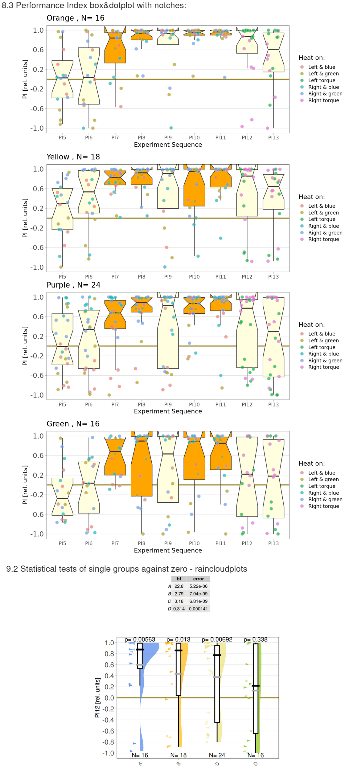
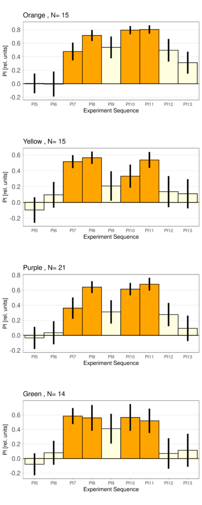
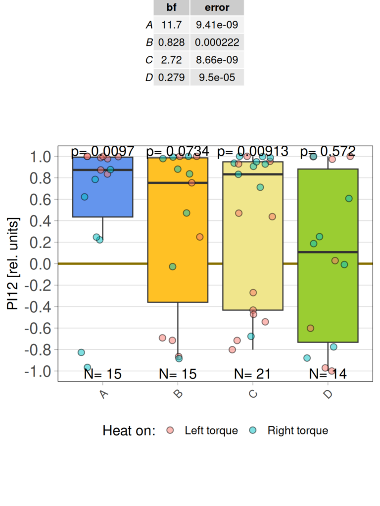
MBON screen progress 19.06.2026
on Monday, June 22nd, 2026 12:15 | by Fridrik Kjartansson

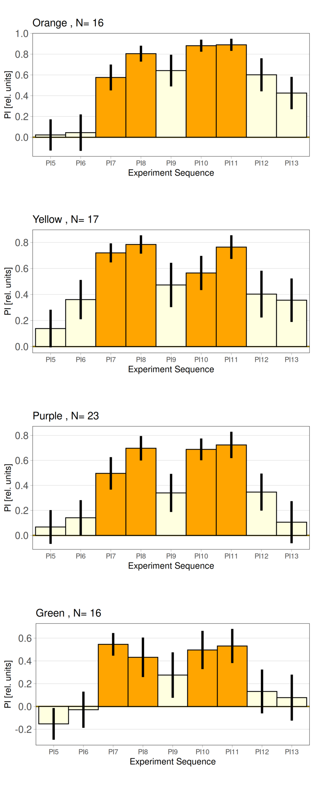
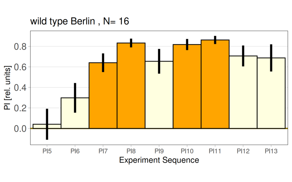
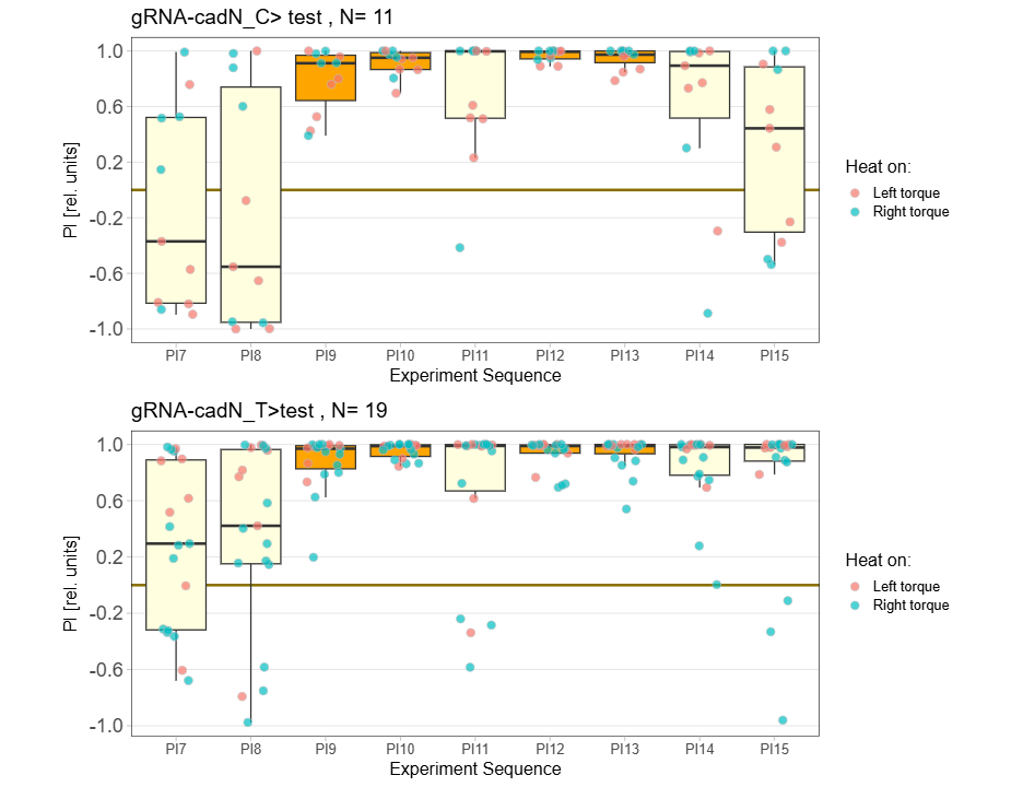
MBON Screen progress 01.06.2026
on Monday, June 1st, 2026 12:59 | by Fridrik Kjartansson
Category: flight, Habit formation, MBON, MBON, MBON, Operant learning, Operant reinforcment, operant self-learning, World learning | No Comments
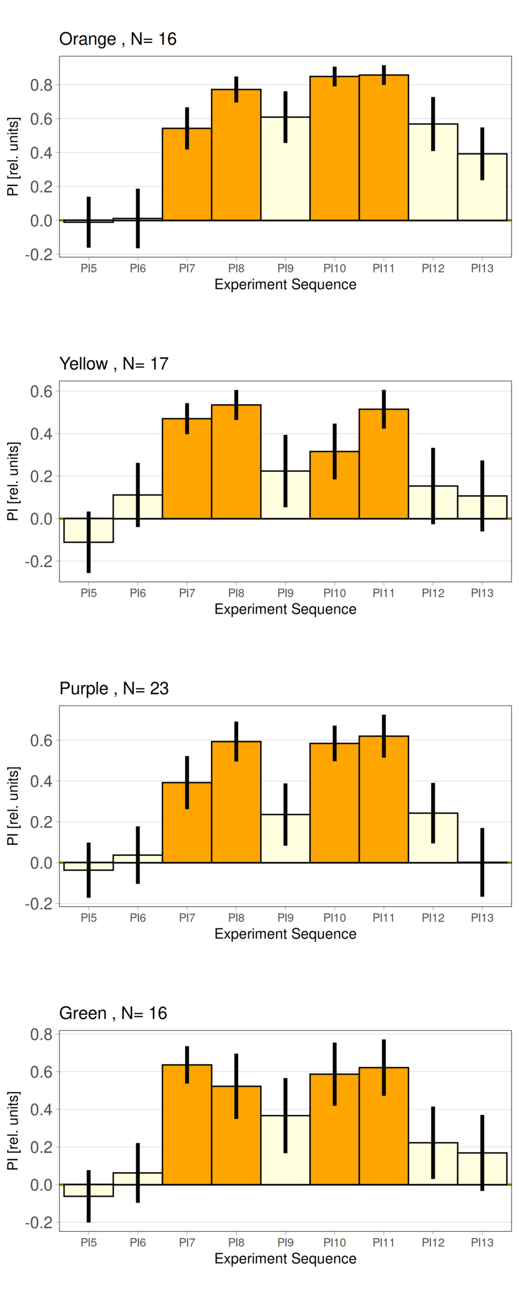
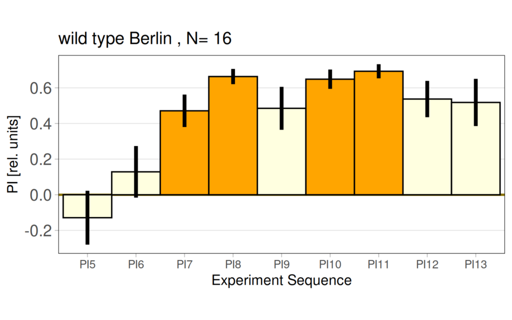
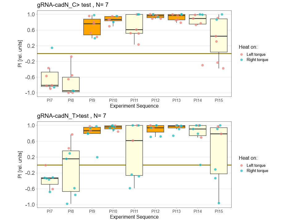
MBON screen progress 18.05.2026
on Monday, May 18th, 2026 12:32 | by Fridrik Kjartansson


Category: crosses, Habit formation, MBON, MBON, MBON, Memory, Operant learning, Operant reinforcment, operant self-learning, World learning | No Comments
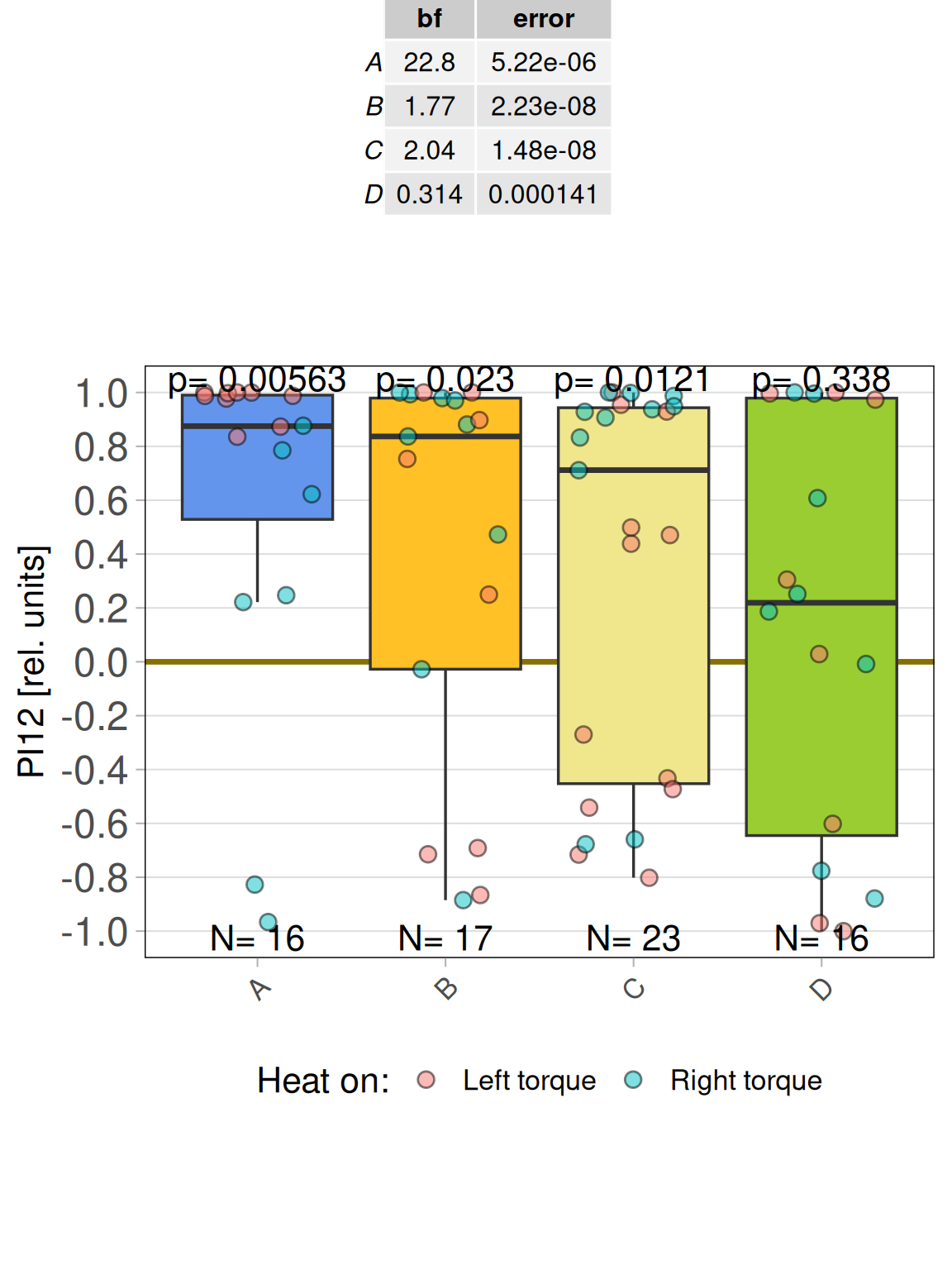
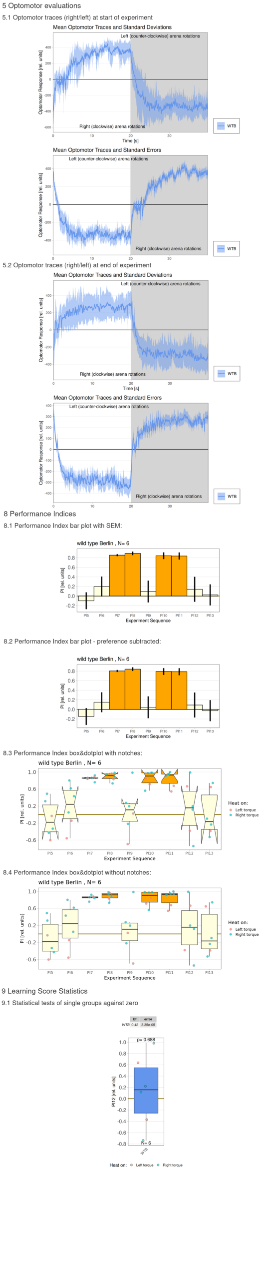
Torque Measurements 24-27.2.2026
on Monday, March 2nd, 2026 4:39 | by Fridrik Kjartansson
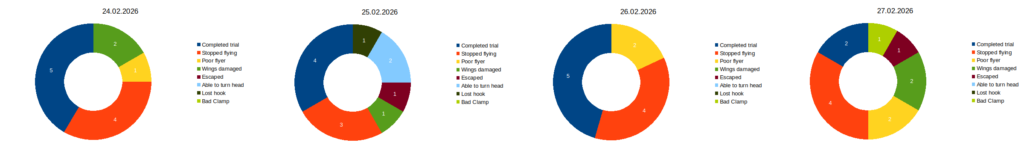
Category: Memory, Operant learning, Operant reinforcment, operant self-learning | No Comments
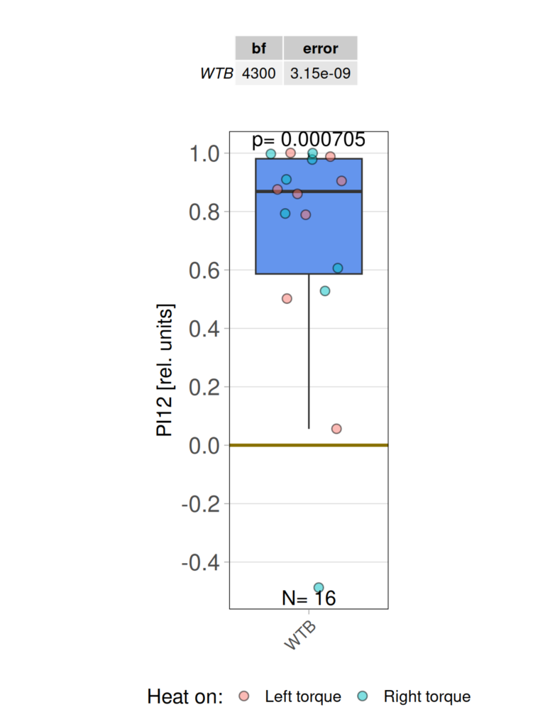
Torque measurements 12.02.2026
on Friday, February 13th, 2026 12:38 | by Fridrik Kjartansson
More data from the basement
on Monday, July 8th, 2024 8:15 | by Ellie
With the modified laser settings I was able to test 3 more wtb. Here are the results:

–> yaw torque
Testing the basement flight simulator
on Wednesday, June 19th, 2024 3:46 | by Ellie
Before collecting the actual data I make sure that the flight simulator in the basement does its thing ;) Here are the test runs with wtb flies for different protocols:

—>> yaw torque

–>> switch mode

–>> habit formation
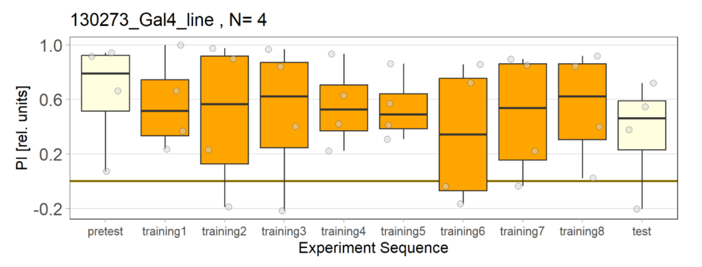
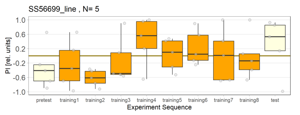
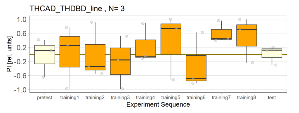
Final ‘Joystick’ test results
on Monday, January 29th, 2024 11:30 | by Devashree Joglekar
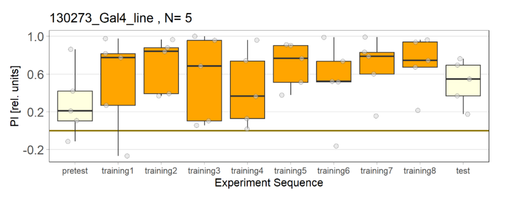
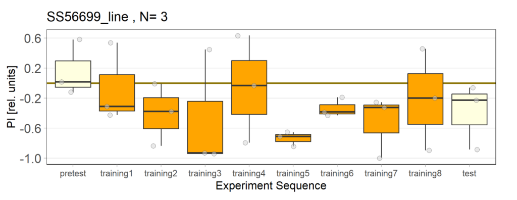
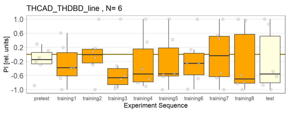
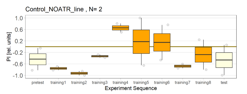
Over the course, control and test lines were experimented with under ‘Joystick’. The test lines include 13:0273-Gal 4 line, SS56699 line, and TH-C-AD; TH-D-DBD line. The tests were done under red and yellow light conditions.
Red light conditions:
Yellow light conditions:

Category: Operant reinforcment, Optogenetics | No Comments