More on valence inference
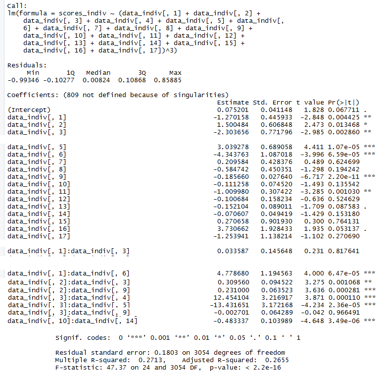
This is the linear model with its statistics

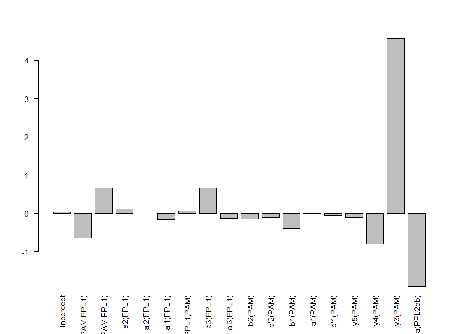
This is the linear model adding interactions. It is perfectly possible to have interactions between neurons, kind of what occurs with olfactory processing where ORNs activated alone or in different combinations have completely different meanings
I uploaded in slack the bayesian linear model with interactions. For any reason, it does not let me upload it now to the website

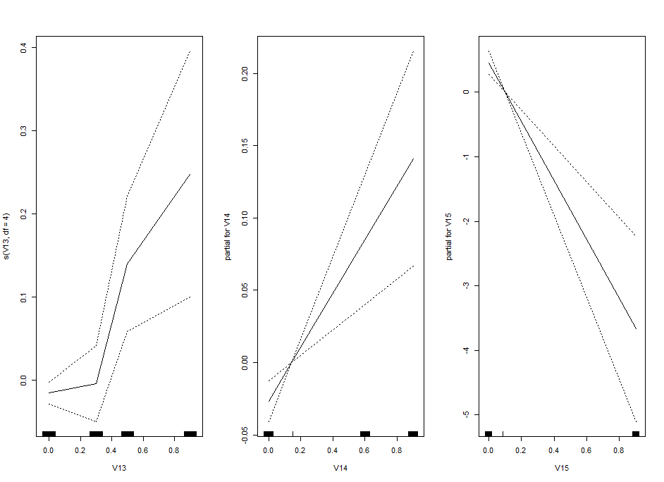
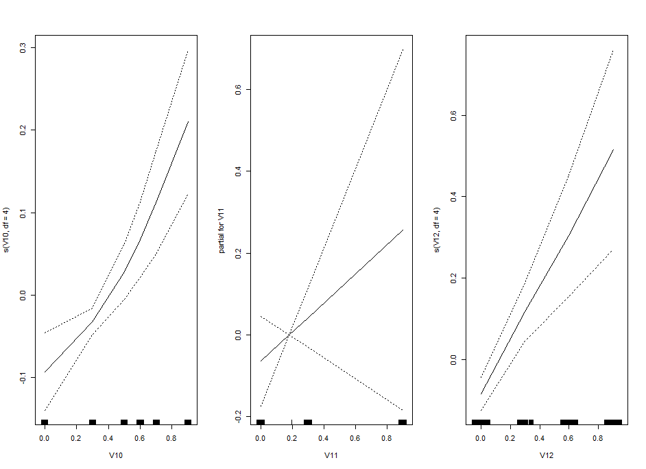
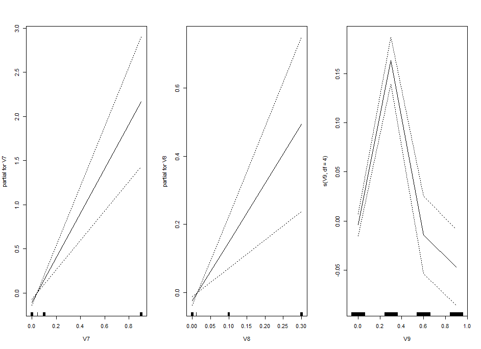
I am trying one of the ways of nonlinear models: GAM (Generalized additive models). Here one fit splines to the effects to certain degrees of freedom.
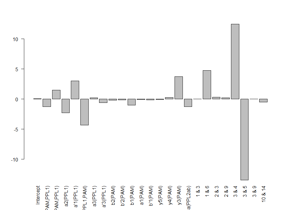
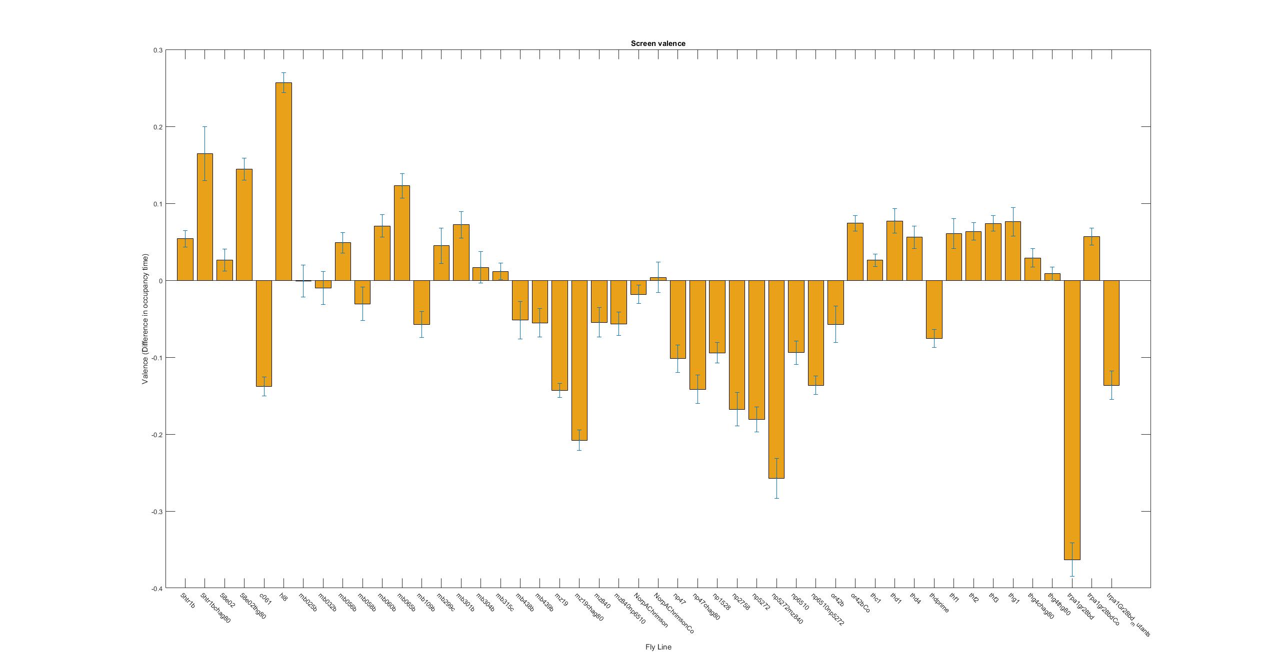
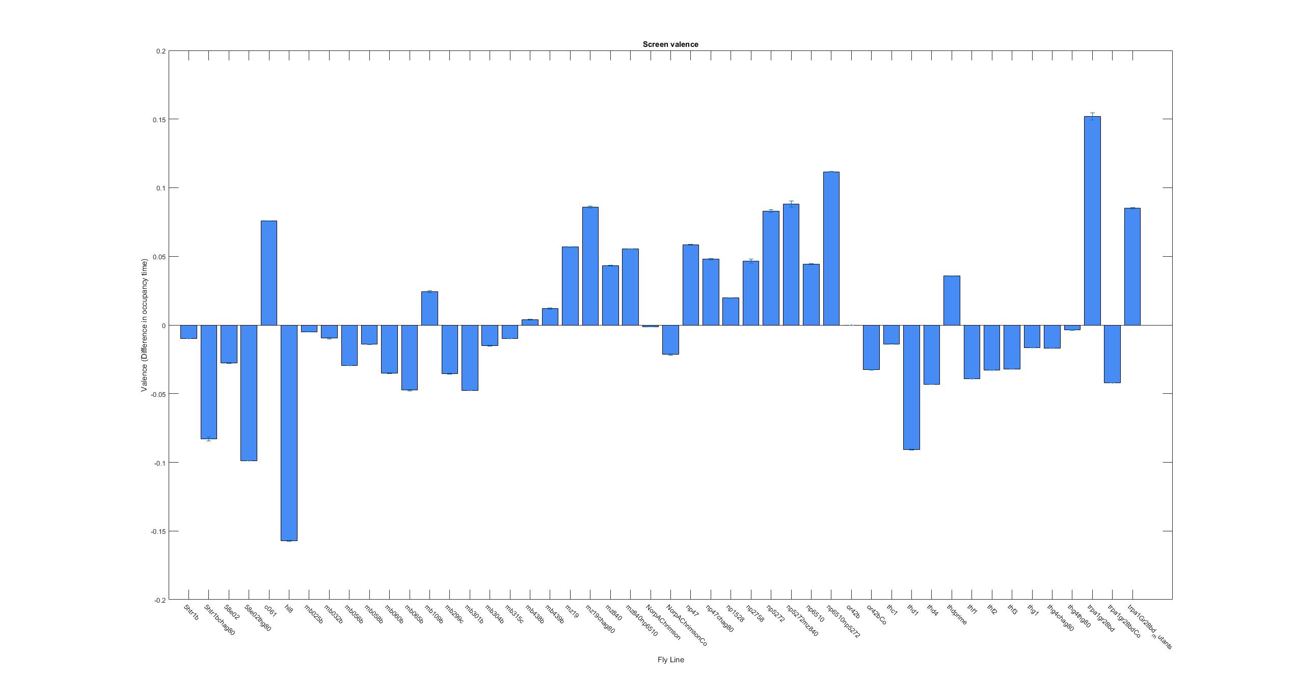
This is the kind of bar graphs I thought I could use for all the plots.

Modelling the valence of dopaminergic clusters from the Y-mazes
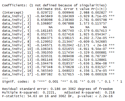
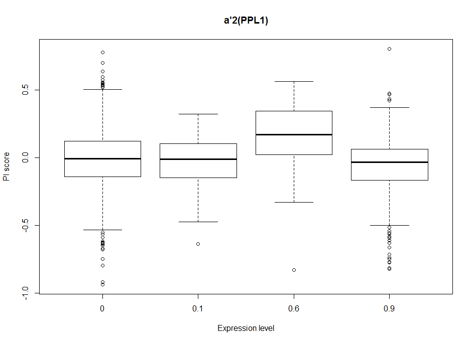
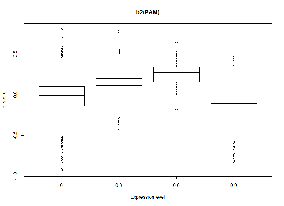
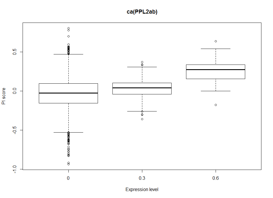
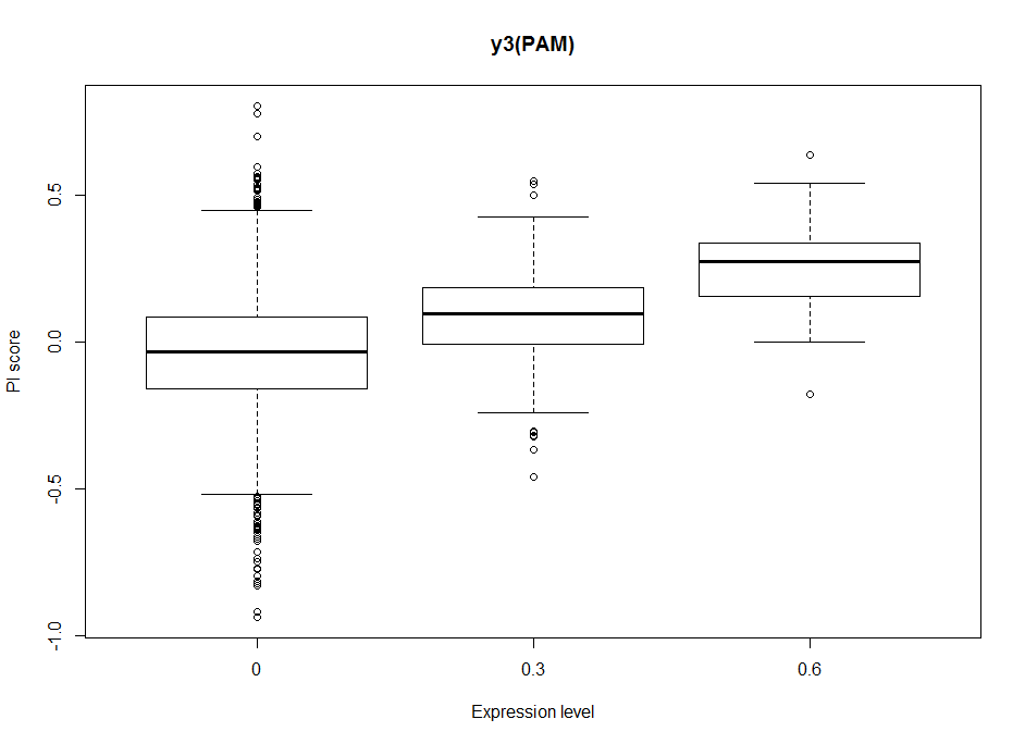
Dopaminergic clusters are differently targeted by the different Gal4s. Some of the express faintly, others stronger. Here I try to see if the dose-response curve (or expression-PI curve) seems to be linear or not. Here I put two examples from the 17 clusters, where the first two seem to have nonlinear curves, with and optimal expression level, and the last two seem to have a linear response curve.
This will be important for the modelling in order to decide to make a linear/nonlinear model. Down below I show the results from a linear model and it´s statistics. From Aso et al. 2012, one could see that activating the lines with TrpA1 shows a linear response curve. But in this case it does not necessarily seem to be the case. Therefore, light intensities might have an effect, as well as the expression level, and conclusion needs to be taken carefully.
In addition it is difficult to calculate this for all the clusters with just one single light intensity test, because not all clusters are expressed in several Gal4s to different level, so that we can estimate from there. So for the interesting lines we might need to make several experiments at different intensities, and see the dose response curve.
The G4s I have used for the modelling are the ones shown here.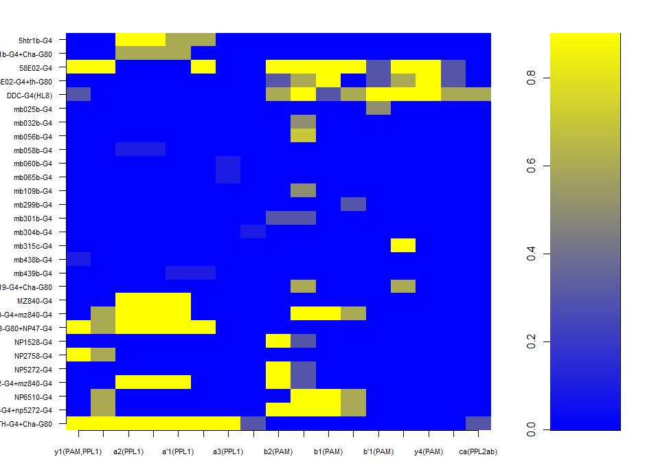
Making new ratios for Y-maze
This is just to show that I am trying to find a new ratio so that all graphs have from -1 to +1 ranges. That is why now the difference in occupancy time is divided by the total time. The same with the speed. Because speed differences are so subtle, the Y axis scale has to be lower
Sathish scripts in my hands are reproducing results
This is a picture of the supplemental figure from Maye et al. 2007
Below the results from the sathish scripts running on the data from Maye et al. 2007. It matches, so Sathish scripts in my hands work fine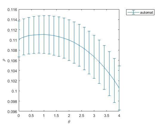
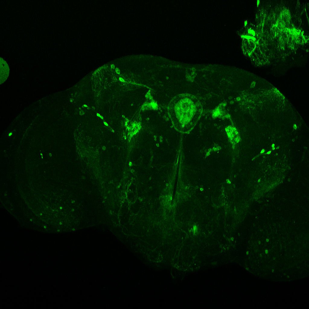
Confocal images and boxplots from my results in strokelitude
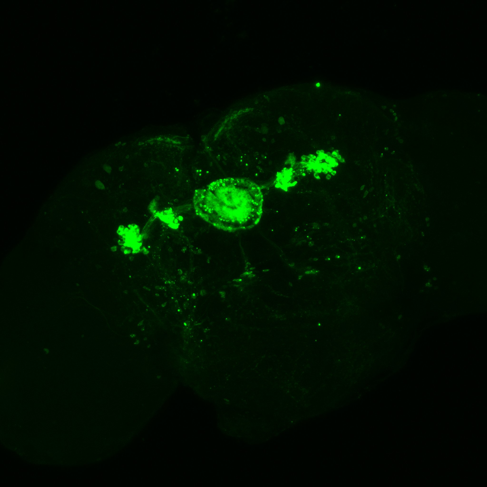
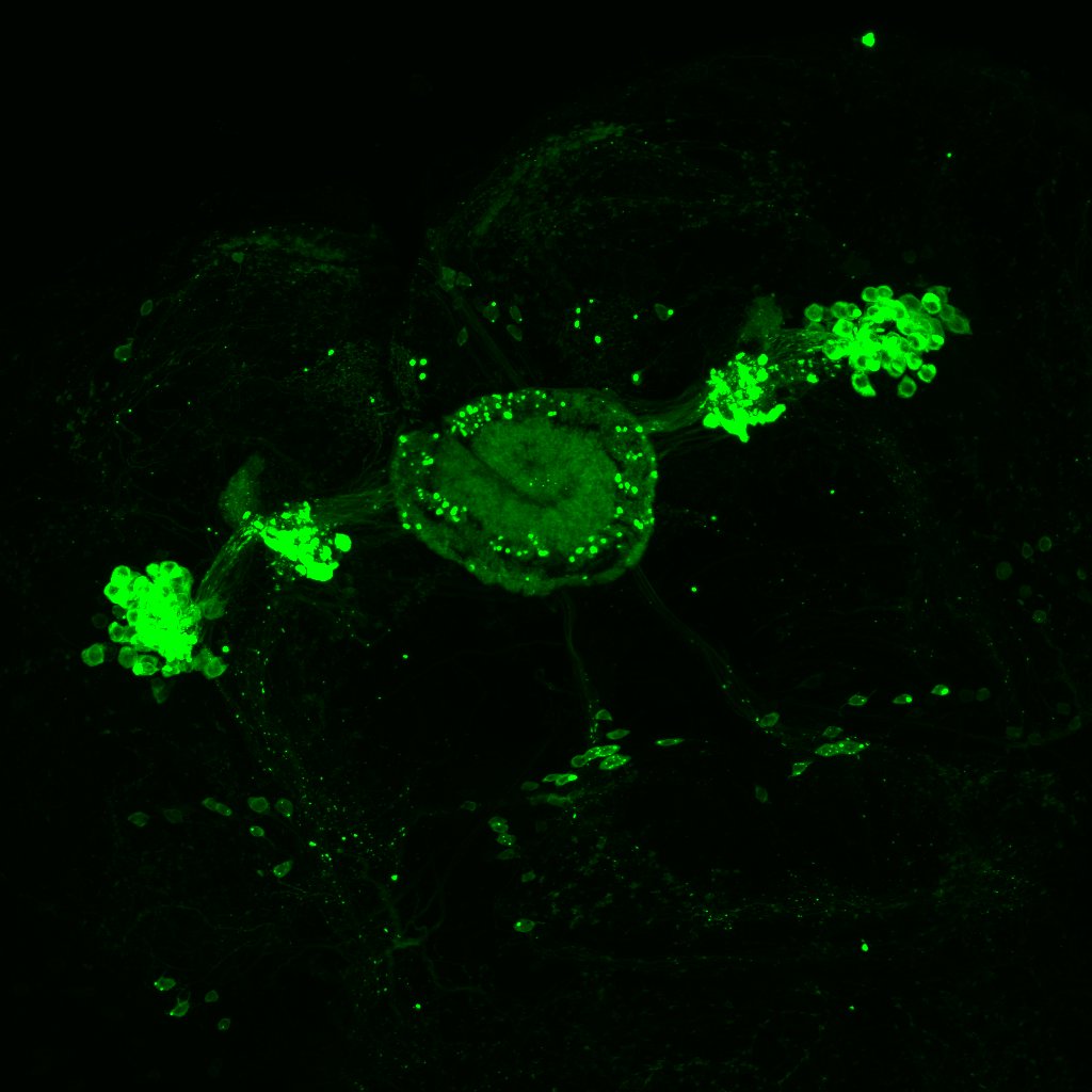
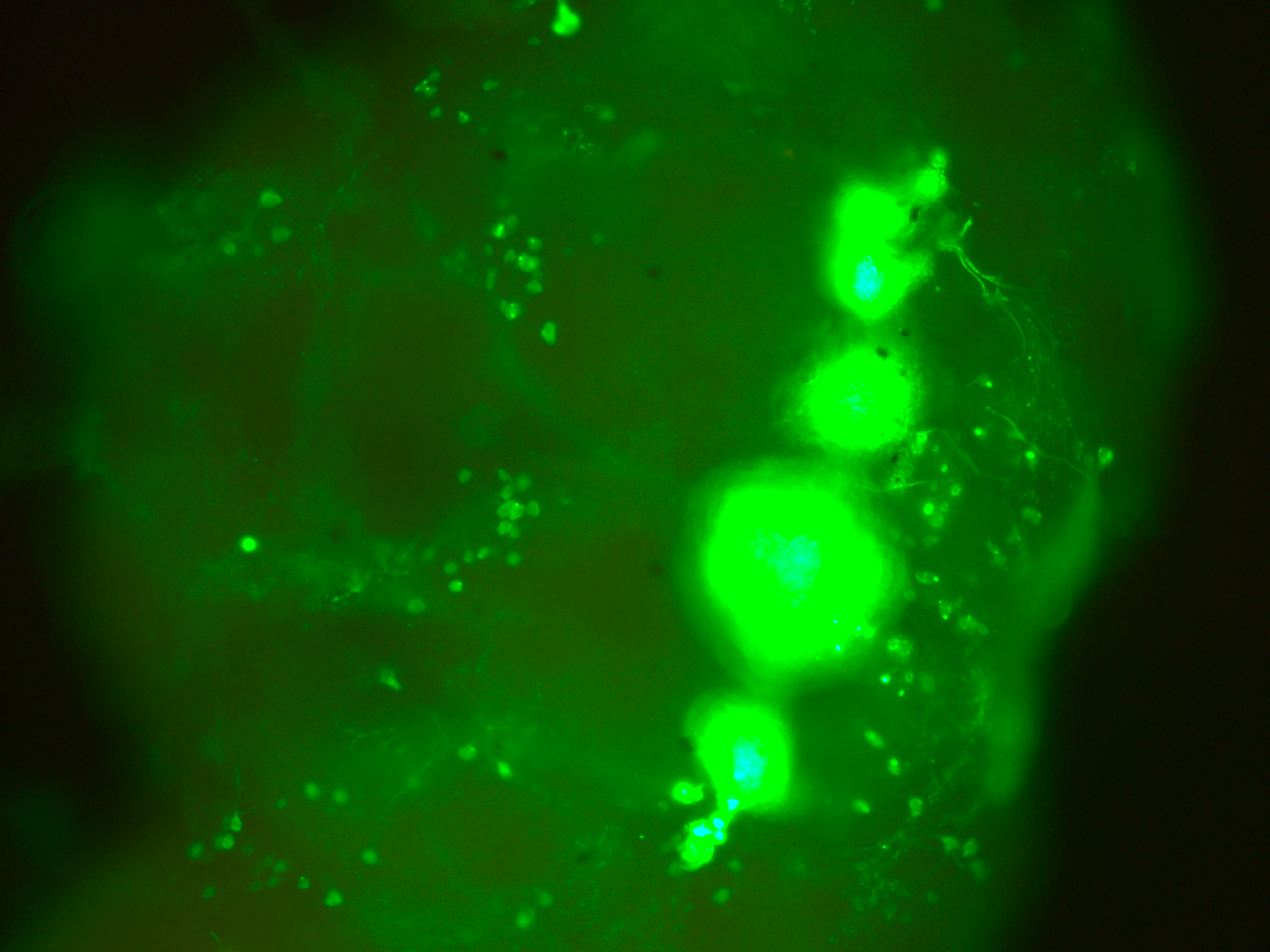
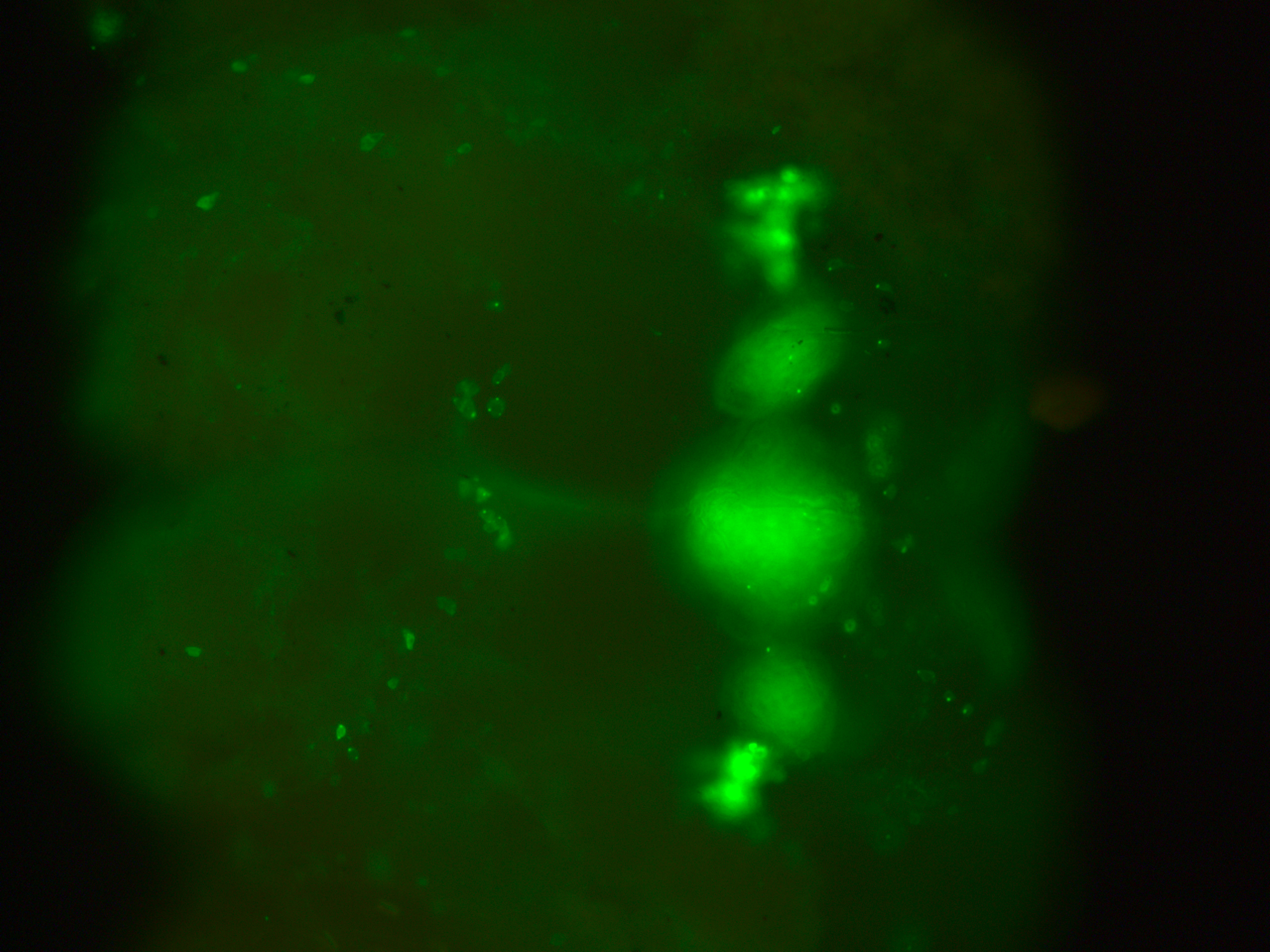
Confocal image MAX stack of one of the brains at 20x
and at 40x
In this link we have a video of a 3D stainning pattern zoomed_CC
In addition I add here teh boxplots from the final results of the Ping Pong ball setup with these experiments 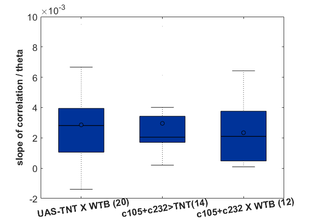
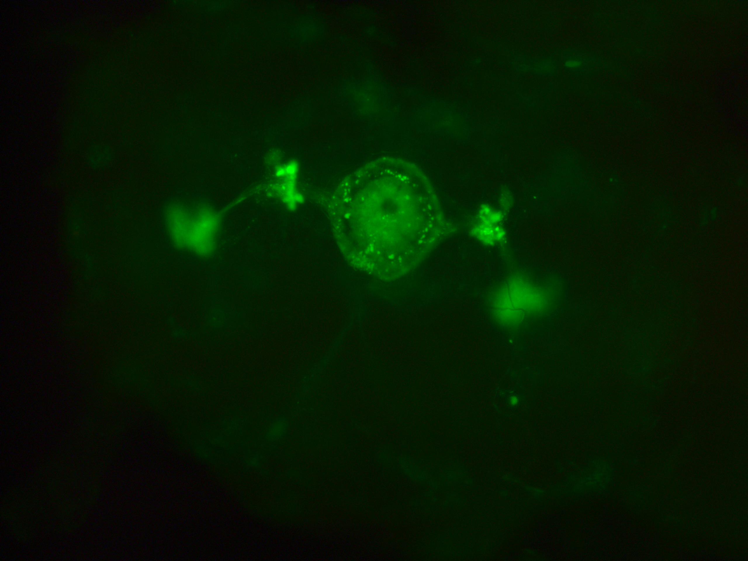
Stainning c105;;c232
The first figure shows each of the central complex ring neurons types (Martín Pena et al., 2014). The c105-G4 targets the R1 neurons and the c232-G4 targets the R2 and the R4d neurons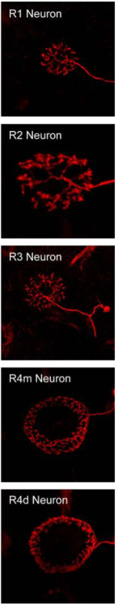
This is the c105-G4 stainning from Martín Pena et al., 2014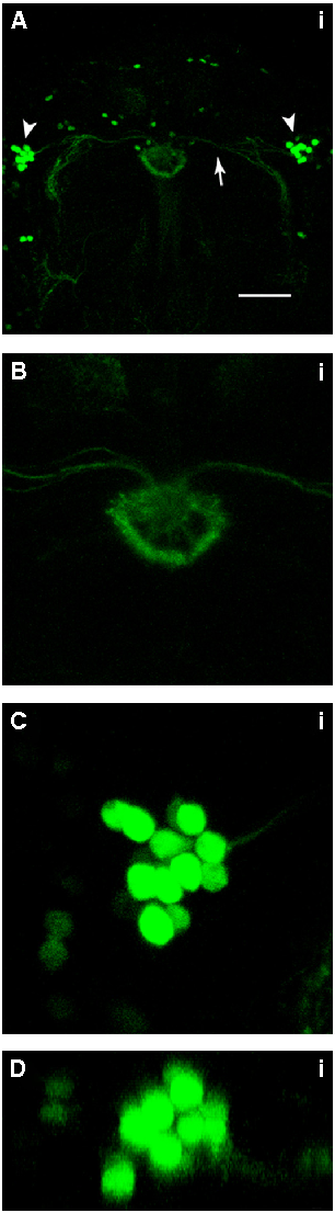
232-G4 stainning from Kahsai et al., 2012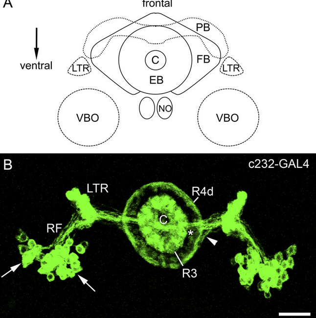
Axel stainning from c232-G4 alone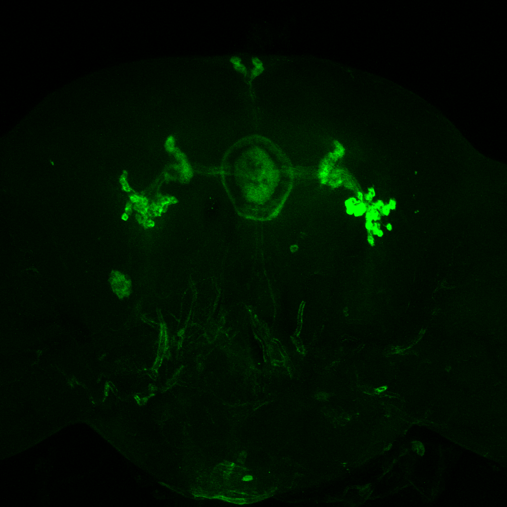
Axel stainning from c105-G4 alone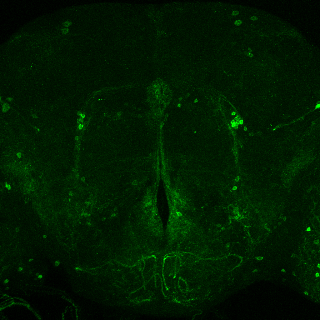
Axel stainning from both drivers together. I would say it really contains both driver lines.
This are both driver lines together as well from Axel. To me it seems that only c105 is present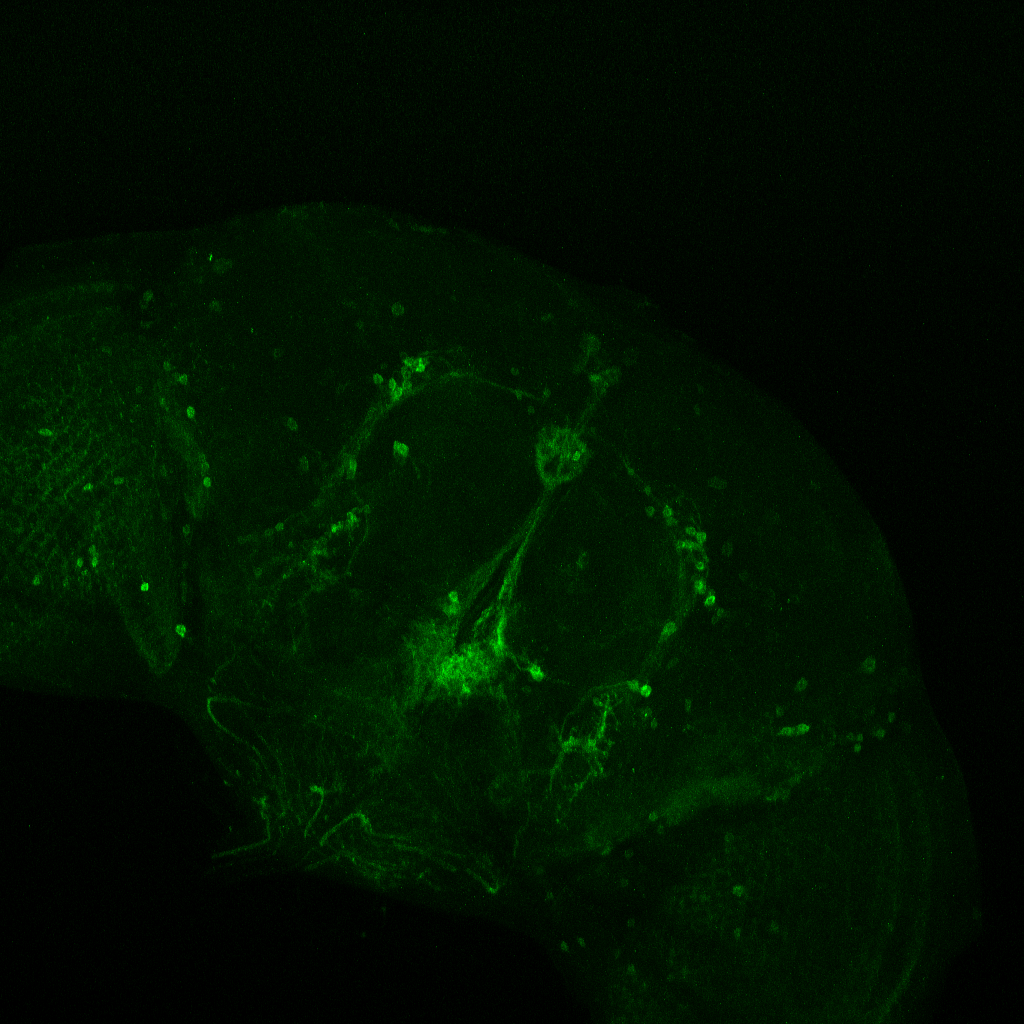
This are my stainnings at the fluorescence microscope (no confocal). This is to show that in all of the 10-12 brains I have looked at, they all had the c232 pattern present
In addition, they had many more neurons outside from the central complex which I believe belong to the c105-G4 line. This is my only proof to show that c105 is also present, since the R1 neurons seem to be hidden when R2 neurons are stained.

I was also looking to the youtube video you have online, Björn. To me it seems I can only see the R1 ring neuron from the c105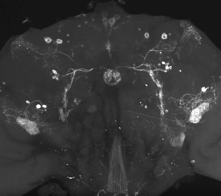
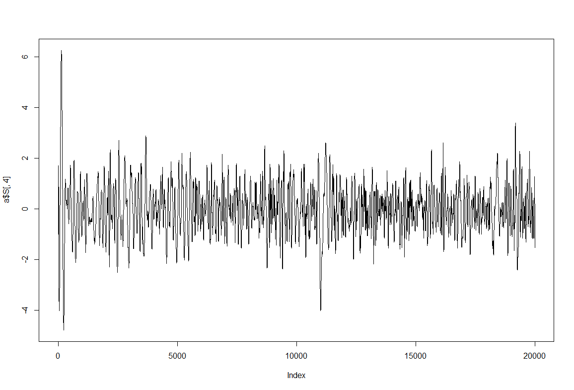
Nonlinearity is present the fast timescales
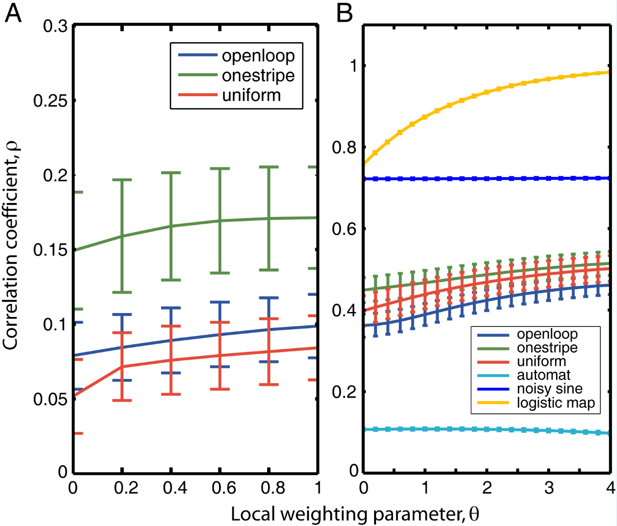
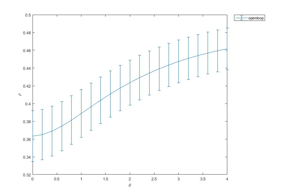
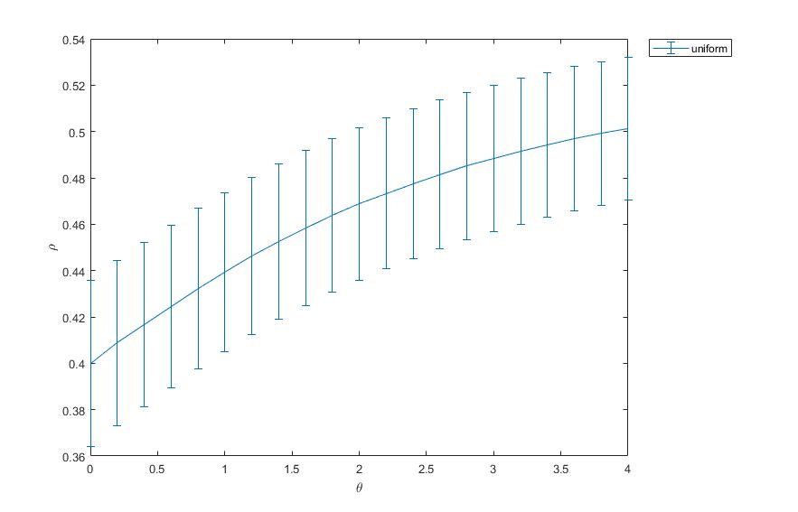
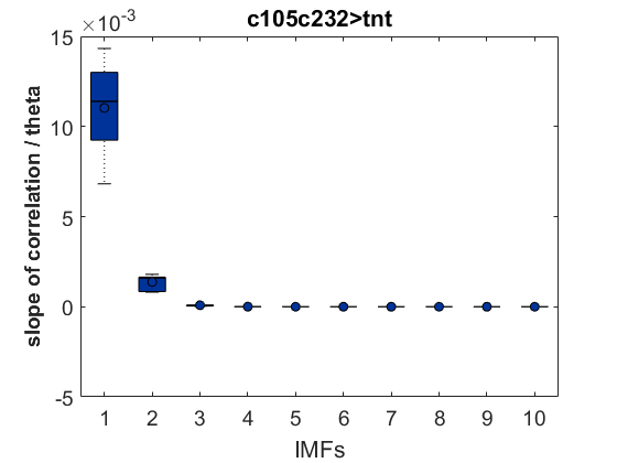
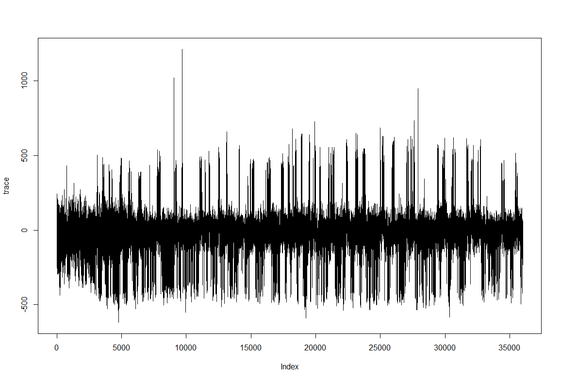
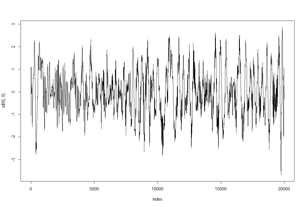
After performing EMD to 6 fly traces of 20000 data points (that is 1000 sec flight) for each group (tntXwtb; c105;c232>tnt; c105;c232Xwtb). This data size was chosen to reduce computing time of the SMAP procedure. The EMD decomposes the trace into different time scales in nonstationary data. It seems that the nonlinear behavior occurs at the first IMF (the fastest time scale) and a bit in the second IMF. The potential conclusion to this is that the behavior of the the fly is only unpredictable at the fast movements whereas slow movements are very predictable. Nevertheless, to be cautious it could be that this fastest timescale is just noise, and that this noise is nonlinear. I would say that there is no difference at any time scale between groups (pay attention to the different ranges in the Y-axes), so the ring neurons R1, R3, R4d do not have any effect. 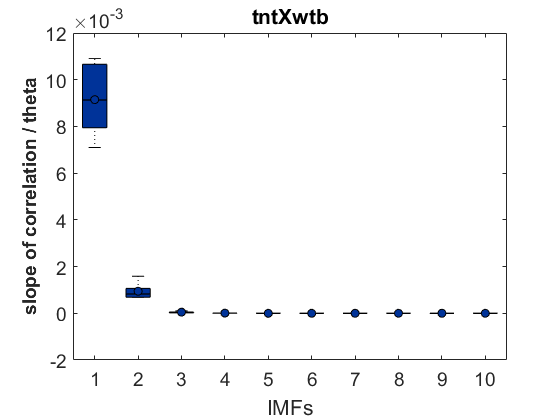
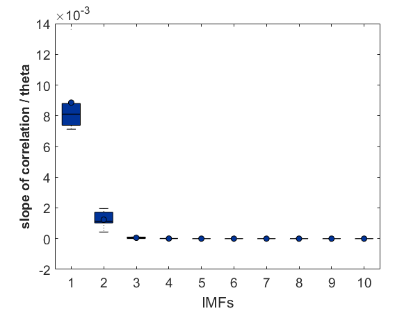
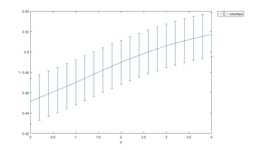
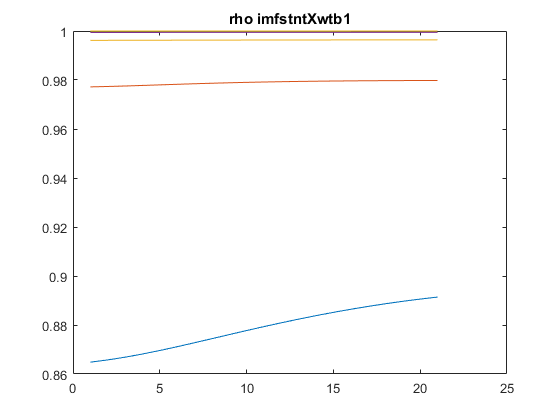
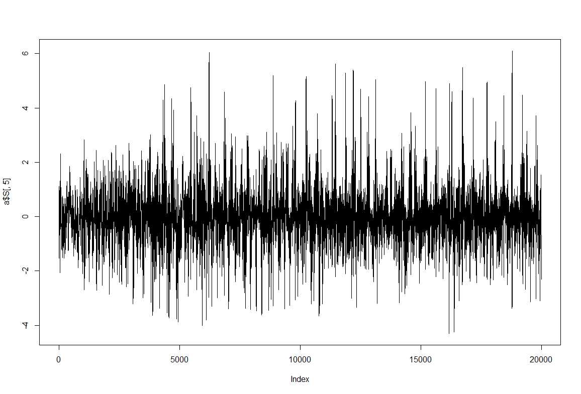
As a groundtruth I have used the same analysis pipeline for the traces in the uniform arena from Maye et al. 2007. Here the effect is even more pronounced at the fastest time scales. So I will conclude that this is real fly behavior and not noise that is shared among both setups: the Ping pong ball machine and the torquemeter. In order to gain more insights into the underlying flight structure I took one random flight trace to explain a few observations. The x-axis is the theta (that actually goes from 0-4 in steps of 0.2 and therefore we see the 21 points), in the y-axis is the correlation of the prediction to groundtruth. We see that IMF has a bigger slope, but not only that, also that its prediction correlation is around 0.88, whereas lower timescales prediction is basically perfect. That is, fast time scales are not only more nonlinear but also less unpredictable. This pattern is repeated in every fly measured
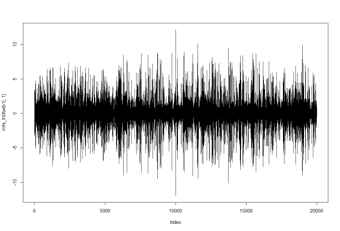
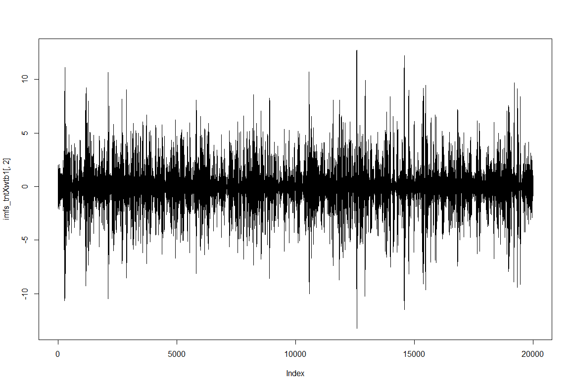
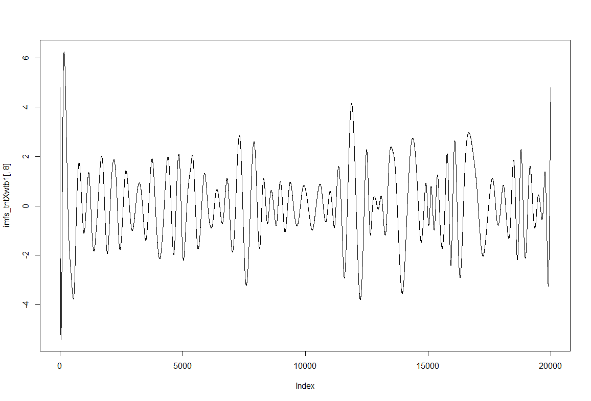
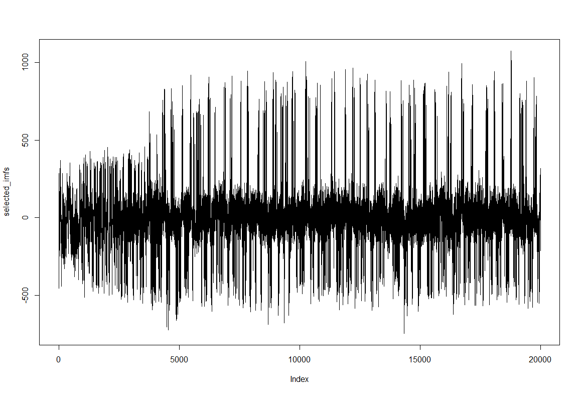
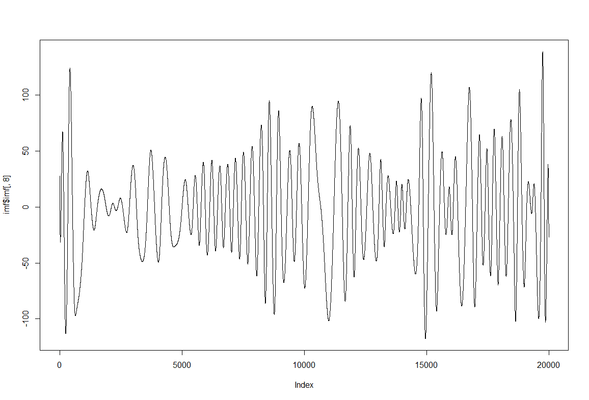
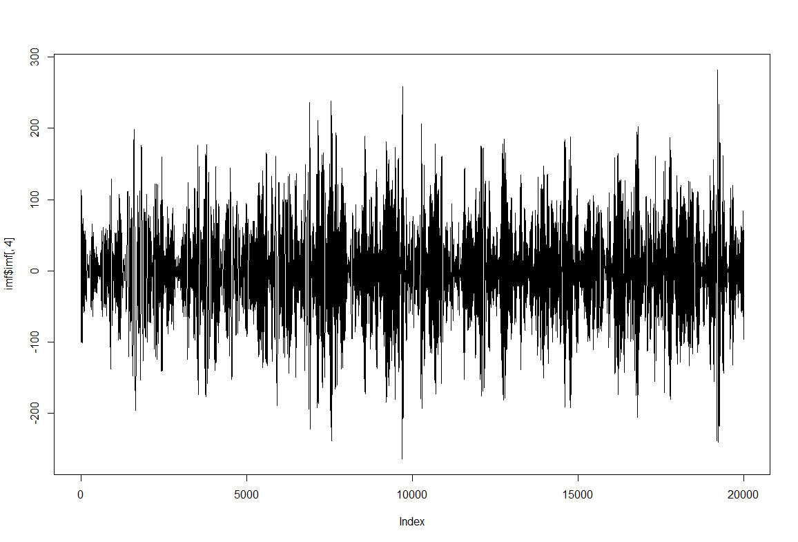
 To have an impression of how these IMF resultant traces look like: IMF1, IMF2 and IMF8
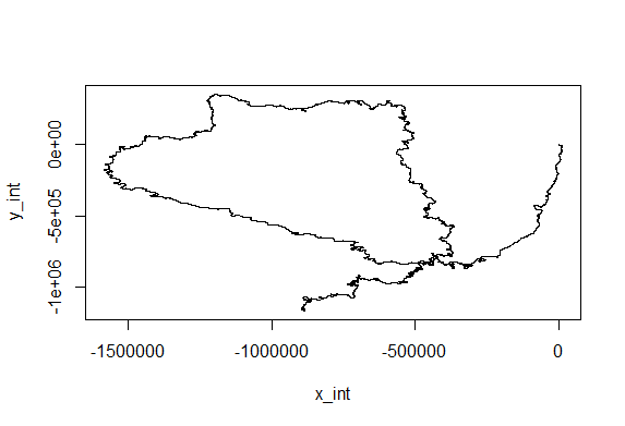
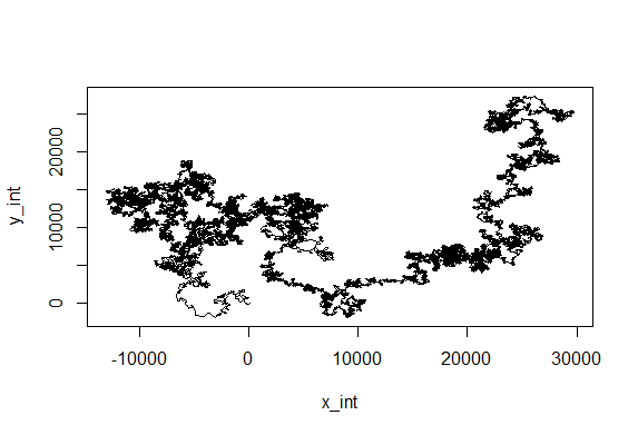
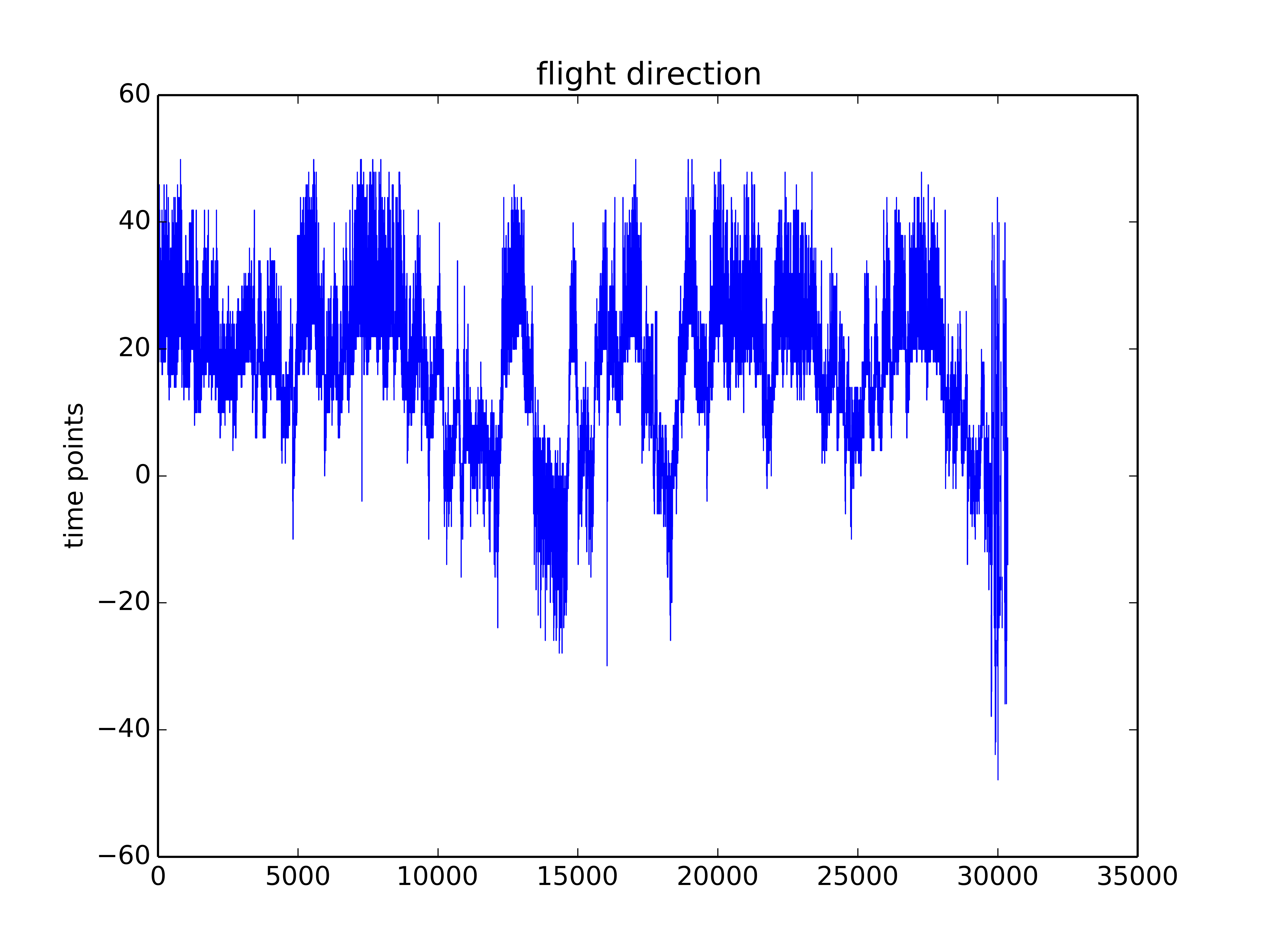
Just creating cartesian traces from polar coordinates
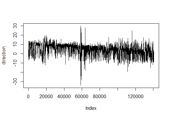
This is for the sake of playing and curiosity. I made out of these two traces a modelling of their flying trace in a 2D world. Direction is right wing amplitude – left wing amplitude and distance flown is dependent on the sum of both (more amplitude of both, more forward thrust). Funny enough, the second one looks kind of fractal, which is characteristic of chaotic behaviors. If there is any comment to add to this new visualization, all ears!
EMD with ICA to one sample of torque trace
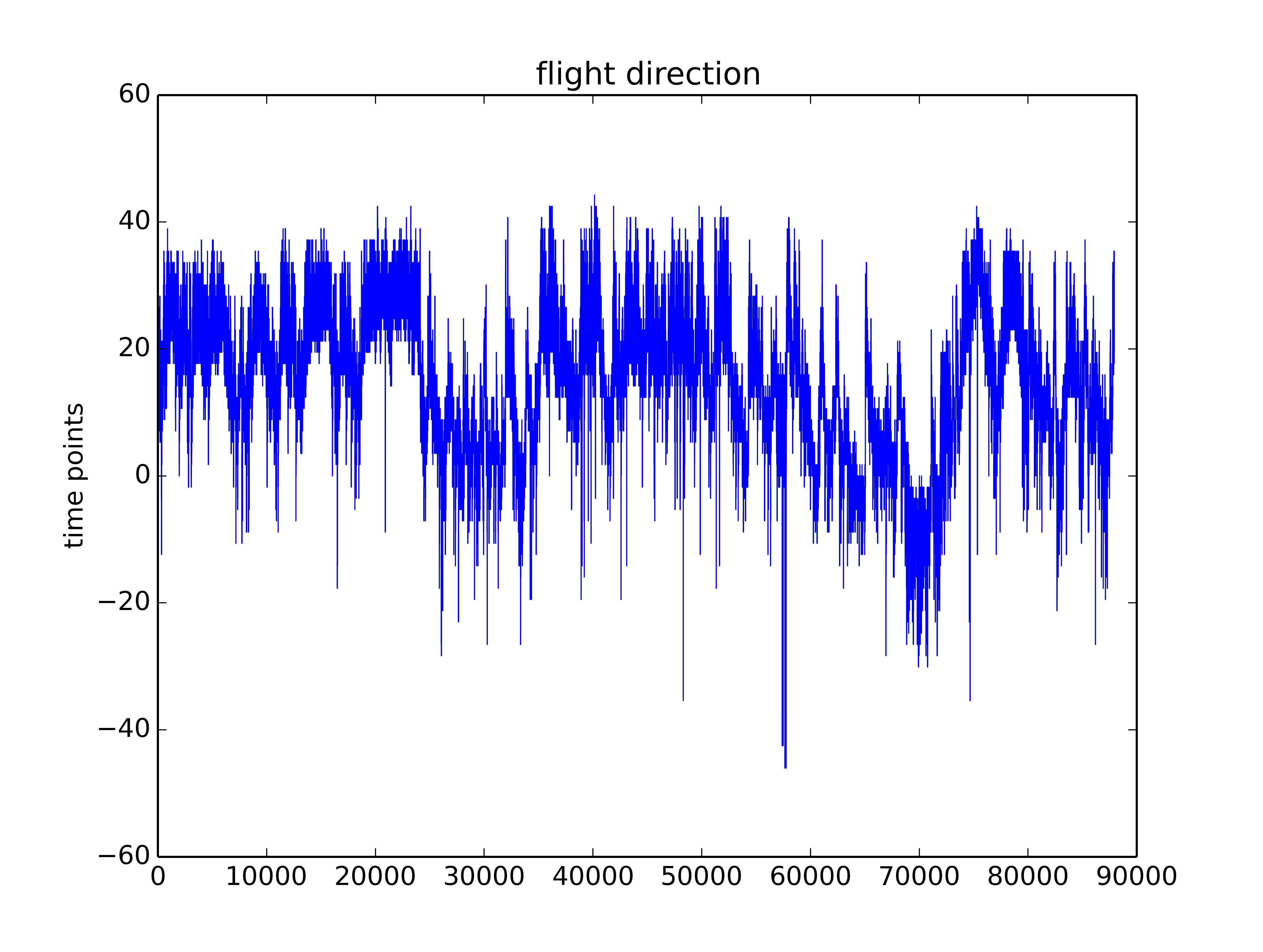
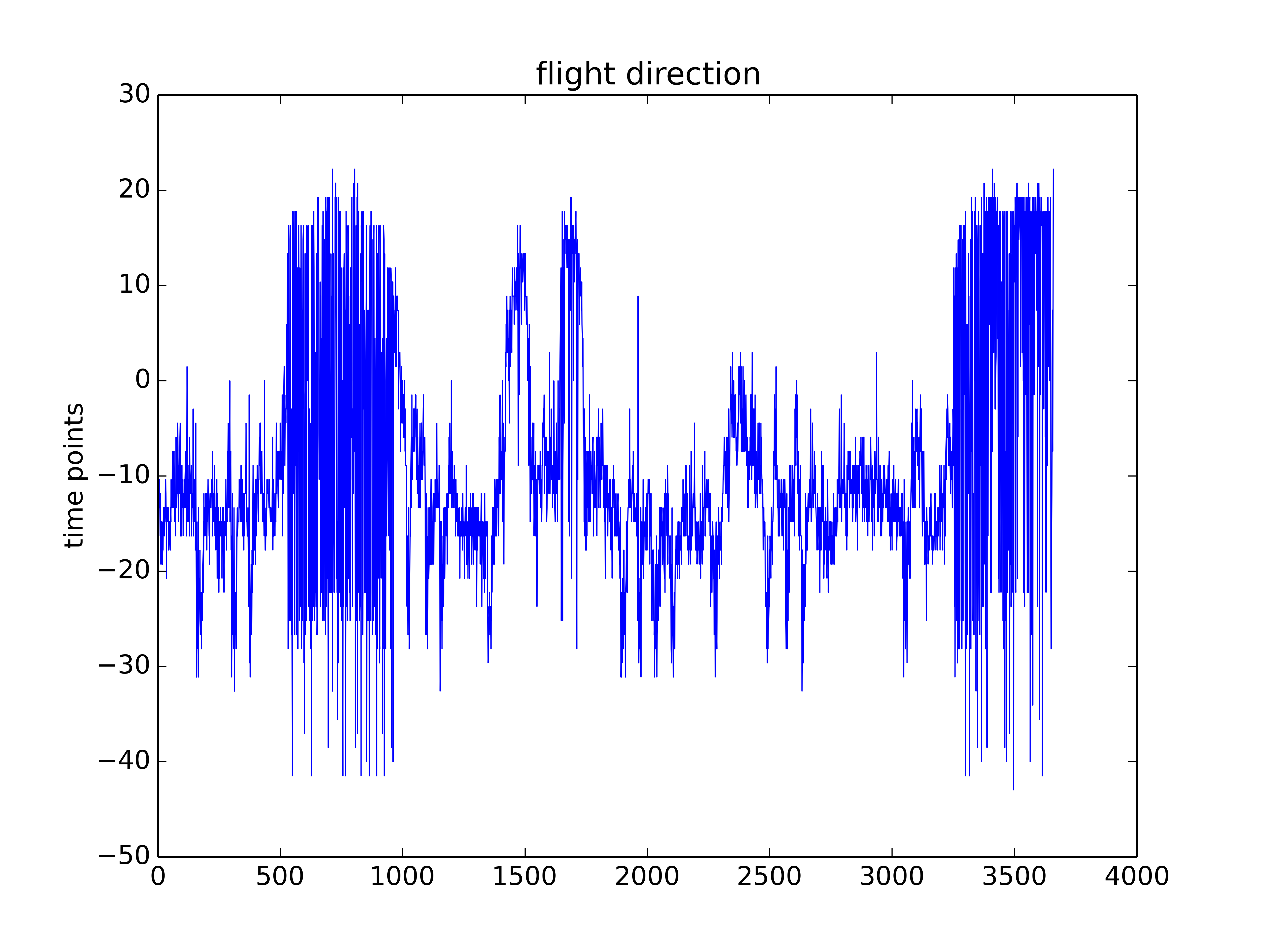
Trace segment from Maye et al. 2007 in the uniform arena
Trace after filtering by selecting the first 8 IMFs (intrinsic mode functions) from EMD (empirical mode decomposition). Since the signal should be quite clean I do not take out the first IMFs. The last IMFs, however, are too slow and change the baseline to much
Some examples of the IMFs obtained from EMD: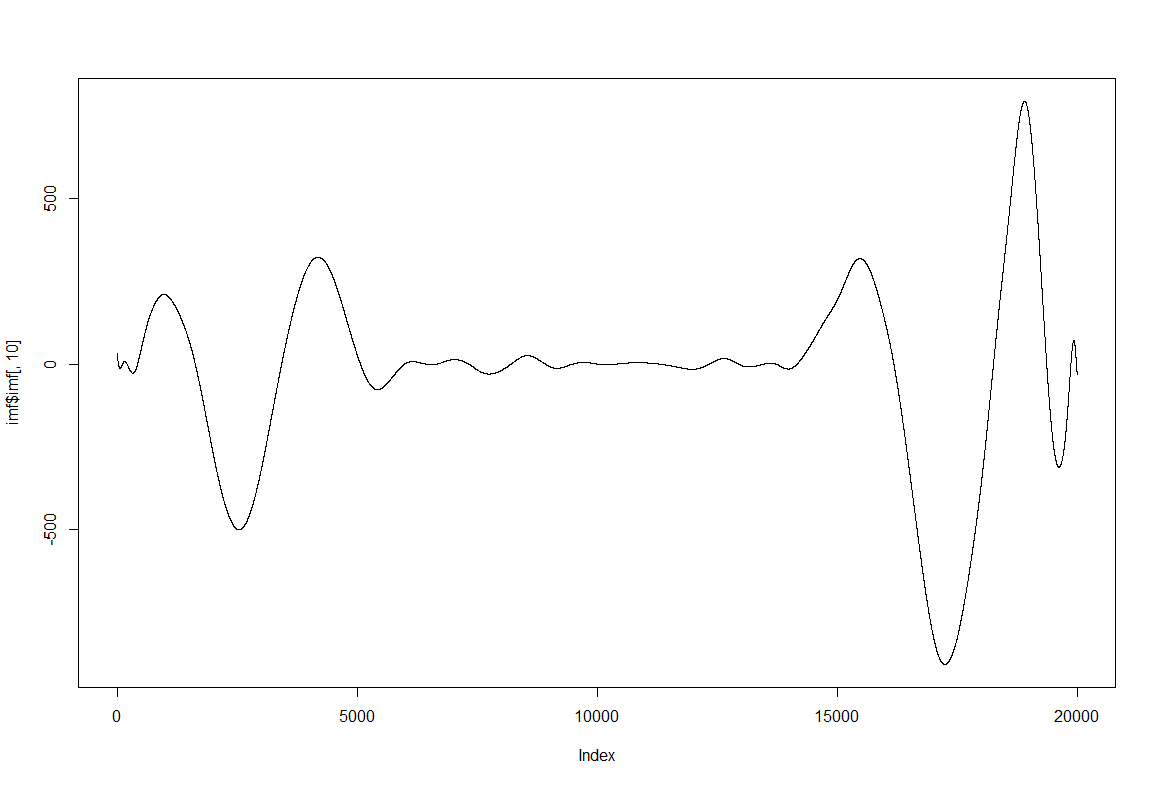
Since this is separating behavior adapting to the data intrinsic time scales I am now thinking of analysing with the SMAP algorithm to see if the behavior is more or less nonlinear at certain time scales.
In addition, I have thought of using ICA (Independent component analysis), that is an algorithm famous for the blind source separation problem by extracting the most independent signals from the input signals (in this case the IMFs which are different time scales of the behavior). So the ICs should consist of mixes of different time scales that are correlated together and thus belong (but not necessarily) to the same action/movement module/… Here a few ICs (from 10). My idea is that muscles might coordinate independently between ICs but coordinated within ICs. However to prove that is not that easy I guess
quality test before strokelitude experiments
 Some traces from this week just so that you have an idea how do they look like. To me they are not the optimal traces I expected. But one can see some signal there. I will start the screen hoping to get enough good traces without too much work.
what do you think is the best quality control for accepting a trace for the analysis or not. I was thinking the 3D mapping gives a good hint but without quantification.
In addition I was writting to Andi Straw to solve the issue of running two cameras in the same computers, but now answer