Wildtype flies and flight simulator
on Monday, June 4th, 2018 9:18 | by Anders Eriksson
The results from wiltype Berlin flies in the flight simulator.

Category: flight, Memory, R code | No Comments
EMD with ICA to one sample of torque trace
on Monday, March 19th, 2018 2:35 | by Christian Rohrsen
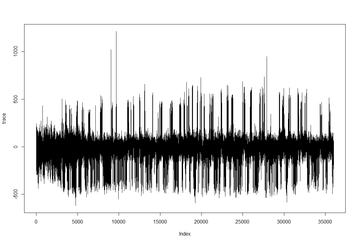
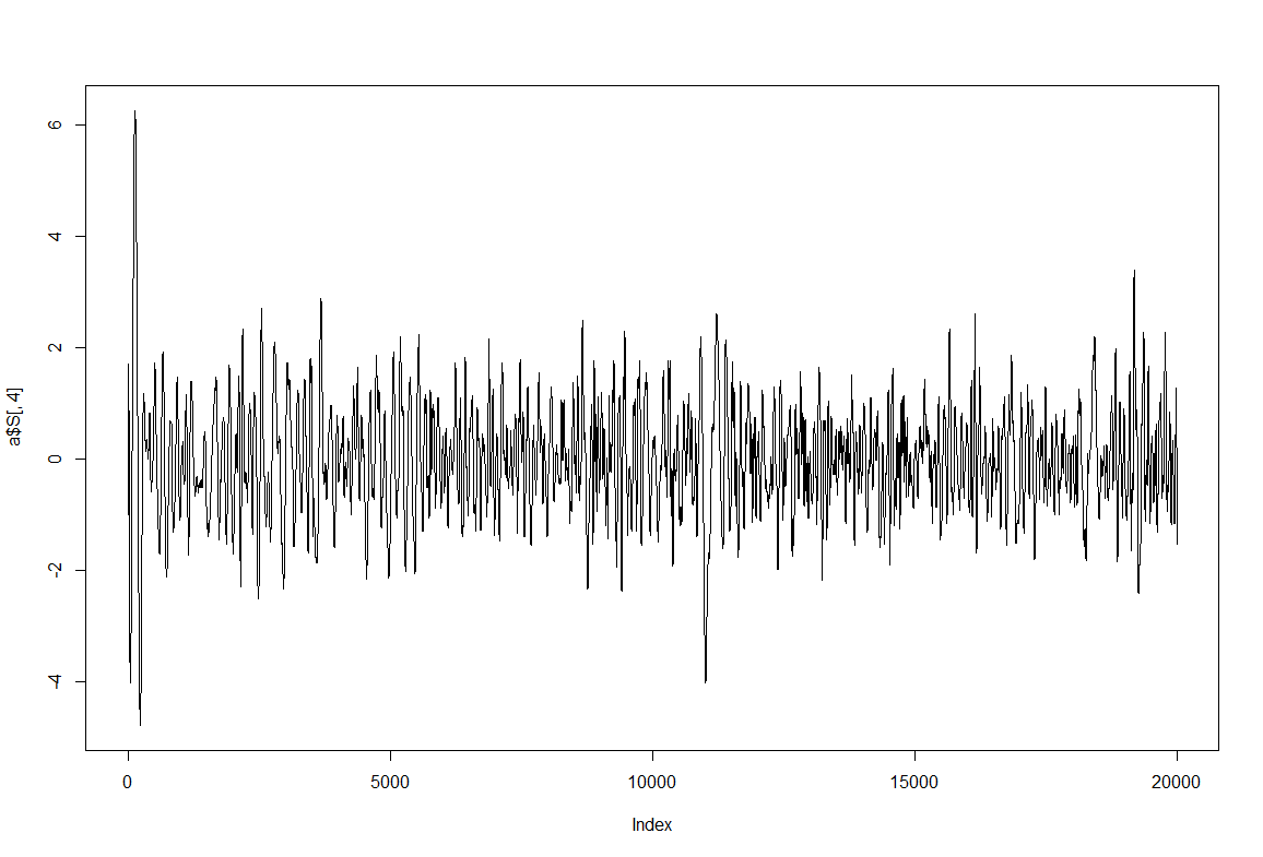
Trace segment from Maye et al. 2007 in the uniform arena
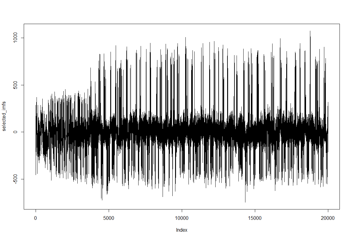
Trace after filtering by selecting the first 8 IMFs (intrinsic mode functions) from EMD (empirical mode decomposition). Since the signal should be quite clean I do not take out the first IMFs. The last IMFs, however, are too slow and change the baseline to much
Some examples of the IMFs obtained from EMD: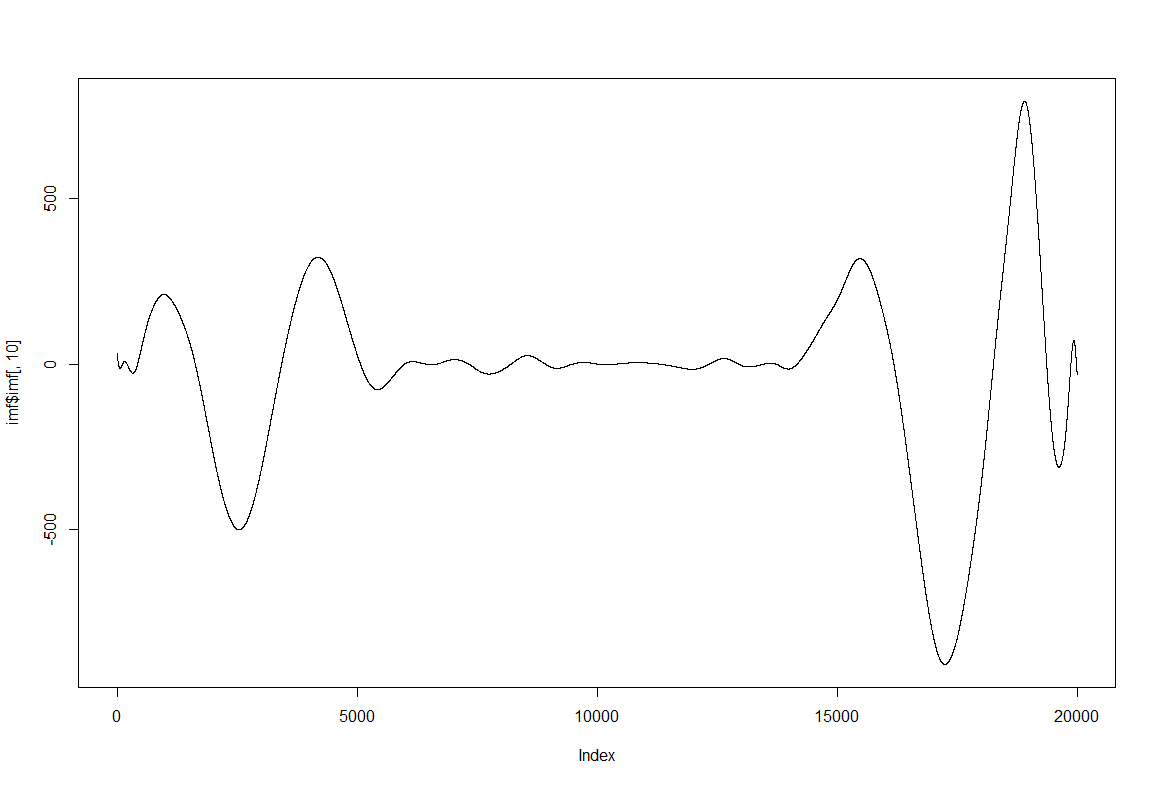
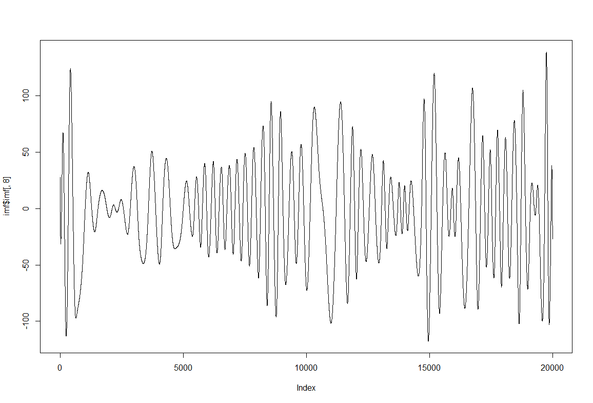
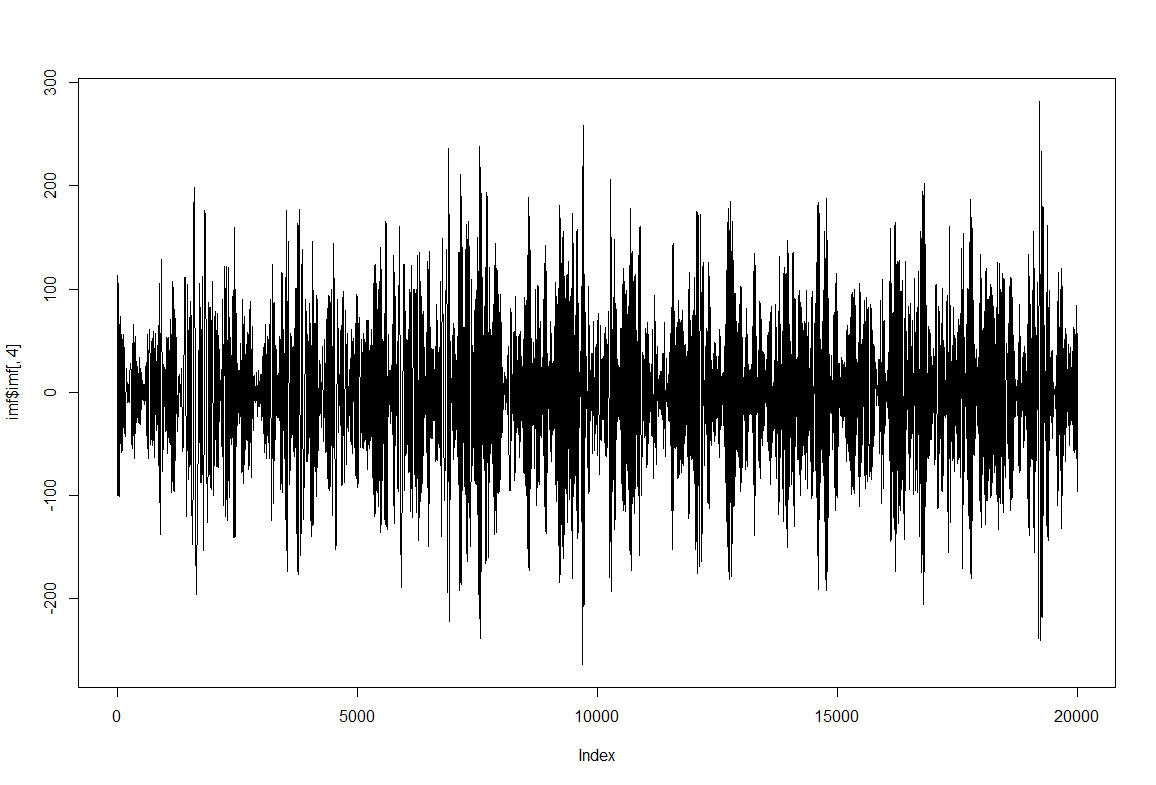
Since this is separating behavior adapting to the data intrinsic time scales I am now thinking of analysing with the SMAP algorithm to see if the behavior is more or less nonlinear at certain time scales.
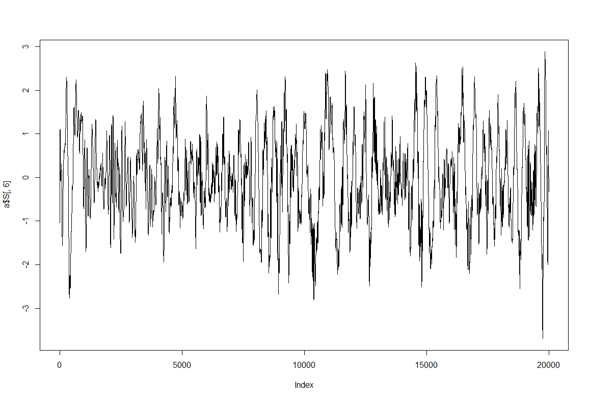
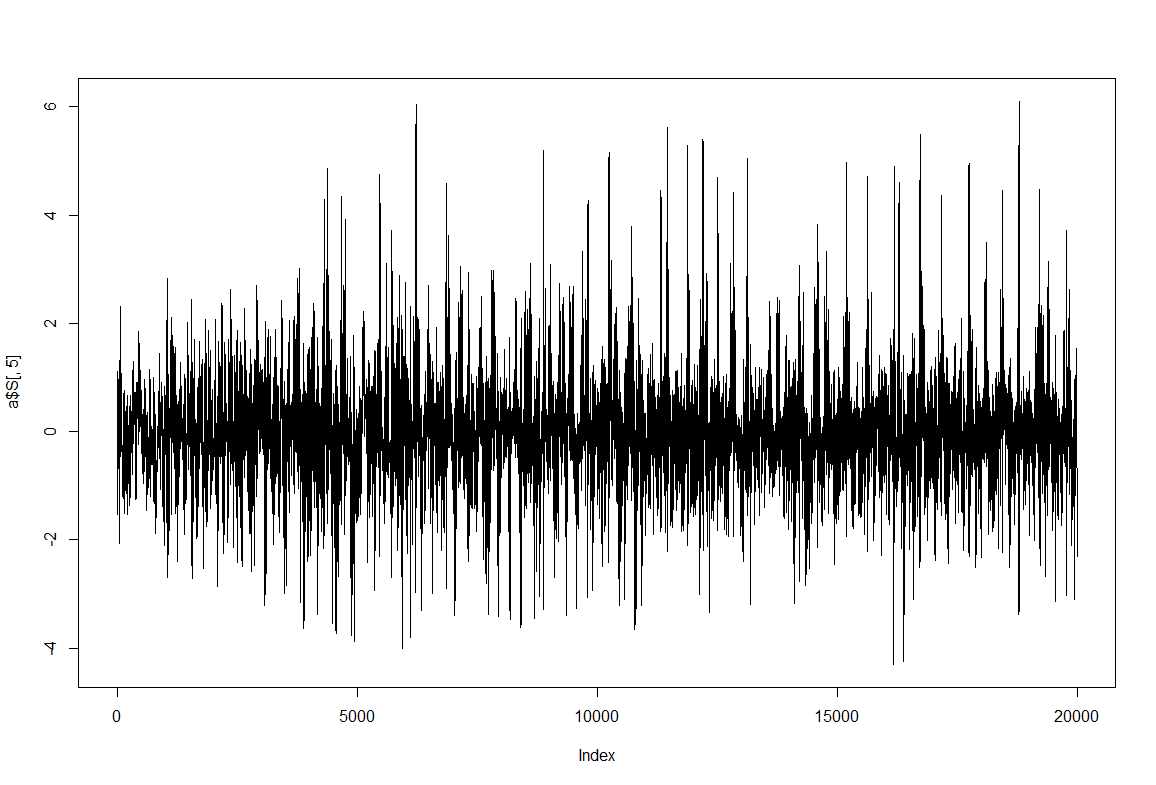
In addition, I have thought of using ICA (Independent component analysis), that is an algorithm famous for the blind source separation problem by extracting the most independent signals from the input signals (in this case the IMFs which are different time scales of the behavior). So the ICs should consist of mixes of different time scales that are correlated together and thus belong (but not necessarily) to the same action/movement module/… Here a few ICs (from 10). My idea is that muscles might coordinate independently between ICs but coordinated within ICs. However to prove that is not that easy I guess
Category: flight, R code, Spontaneous Behavior | No Comments
SMAP results
on Monday, October 9th, 2017 2:34 | by Christian Rohrsen
These are the results of the SMAP for the TNTxWTB. I also have done a few for the c105;;c232xWTB but there is not much to say. I would say that the cleanest lines show a bigger slope, but prone to subjectiveness.
In addition, I have done some animations of the attractors that I have posted on slack because of size.

Category: flight, genetics, R code, Spontaneous Behavior, strokelitude, WingStroke | No Comments
Droso Kurs and more
on Friday, April 22nd, 2016 6:18 | by Christian Rohrsen
Here I attach the results in a pdf file from the students praktikum with an additional line I tested on my own meanwhile (Gr28bd and TrpA1 drivers together). They seem to work as a really good positive control btw, good for technique optimization.
For the students I tried out two different split drivers, the MB058B, which targets PPL1-a’2a2, and MB301B, which targets PAM-b2b’2. In addition the Gr5a driver, because it targets the “sugar” neurons. From the split drivers I wanted to see if I still get a validation from my initial model. MB301B seems to do quite what my model would predict but MB058B maybe not. Hopefully in a future screen I would be able to test many more and make a much more precise modelling.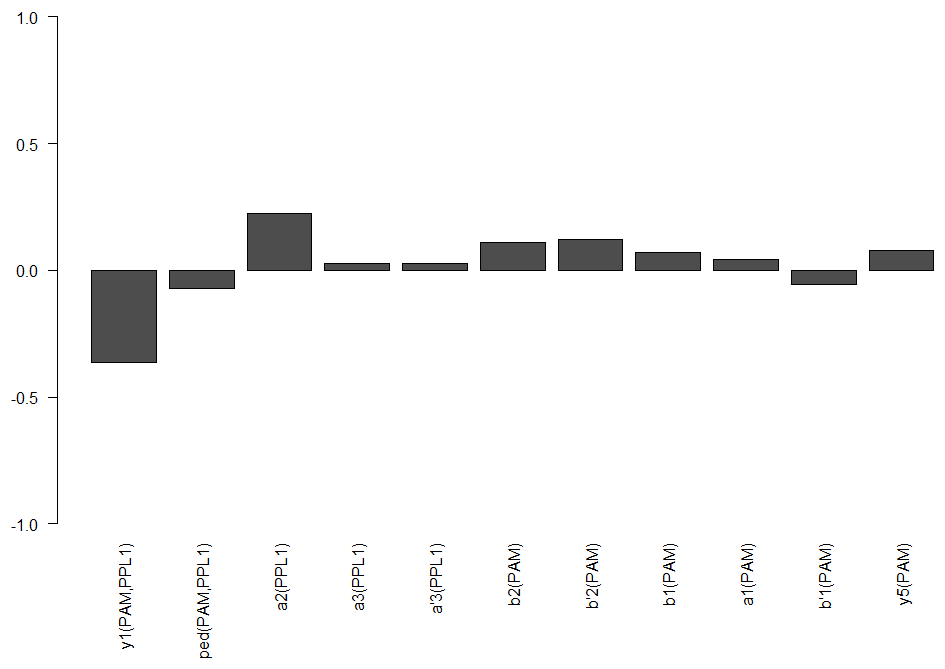
Category: neuronal activation, Optogenetics, R code | No Comments
Cumulative bins, starting at zero and normalizing
on Monday, April 4th, 2016 3:04 | by Christian Rohrsen
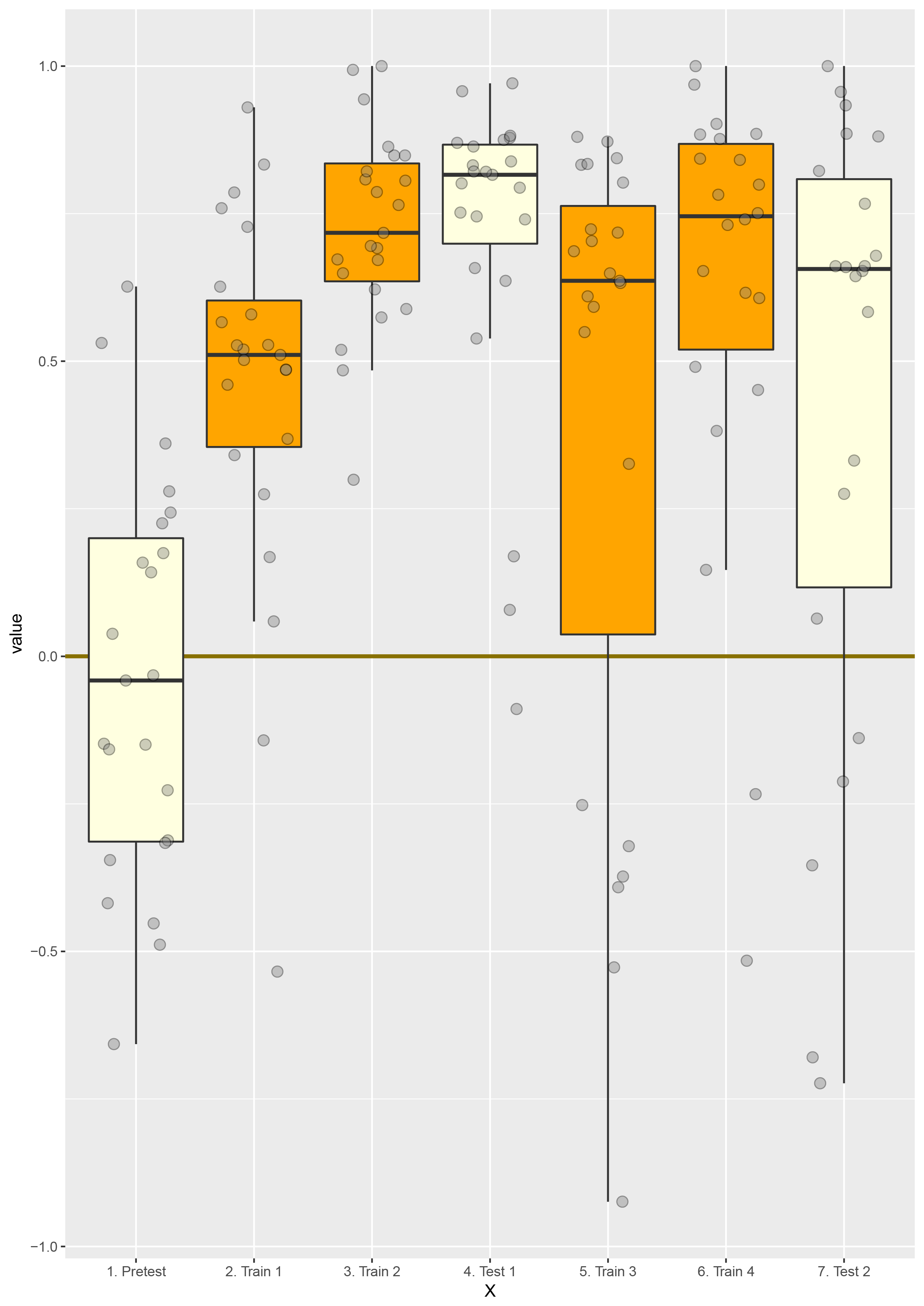
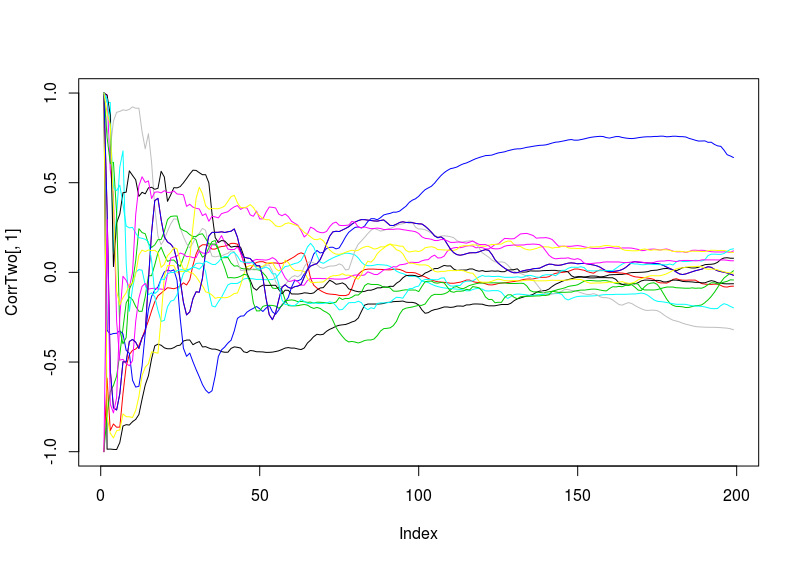
In the last meeting Björn proposed to do correlations of cumulative increasing bins. He said to do that taking the zeroth point (last library point where prediction is still not done) and use it for having a potential 1 of correlation coefficient at the beginning. I could not do that because I didnt save the zeroth points, and this will be a bit tedious and confusing considering that many flies were tested and probably the order is not 100% known. Thus, I just did the bins skipping this zeroth point. After all, we should see something similar with this one. First two graphs: c105;;c232>TNT (first and second prediction point), second: WTBxTNT, third: WTBxc105;;c232.
Examples of how each of the flies look like. So they are basically cumulative bins with each single fly (each in different colour). Just to have a hint how does the singularity looks like. 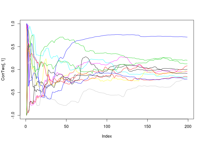
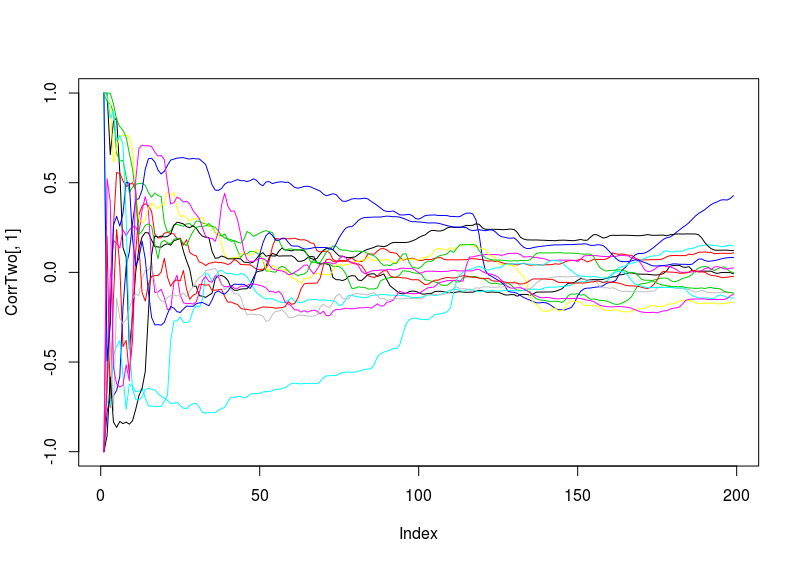 Second thing I did is normalize the to have a range from -1 to 1 all of them (I have to double check the range in the script) and also setting them at a starting point of zero. I did this because we do not want to have differences in the correlation coefficient due to a different offset of the values of the wing beat and neither because of the starting point (if the fly was already flying to the right full gas, then it could be that it has an influence in the following prediction).
c105;;c232 –> first at starting at zero without normalizing and then with normalizing. The next is just the RMSE (not so important).
Category: R code, Spontaneous Behavior, strokelitude, WingStroke | No Comments
Prediction with binnning
on Monday, March 21st, 2016 1:13 | by Christian Rohrsen
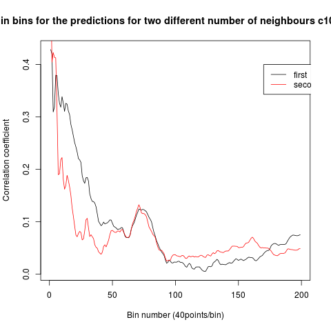
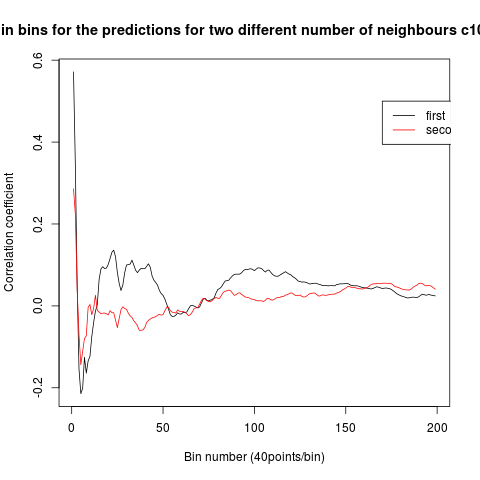
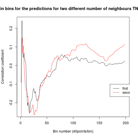
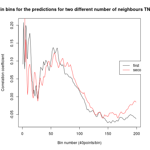
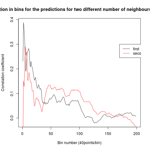
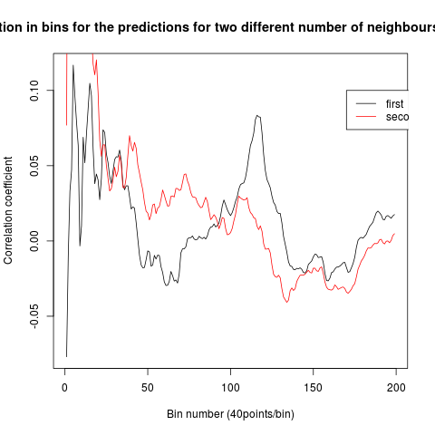
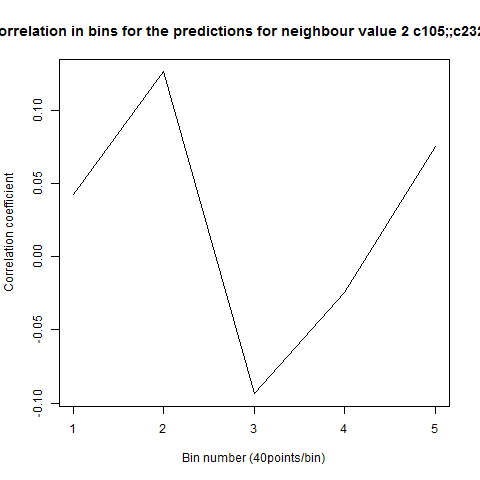
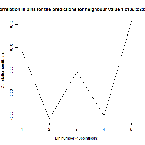
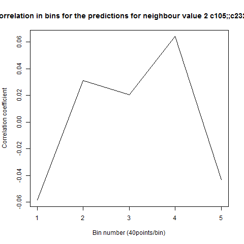
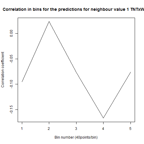
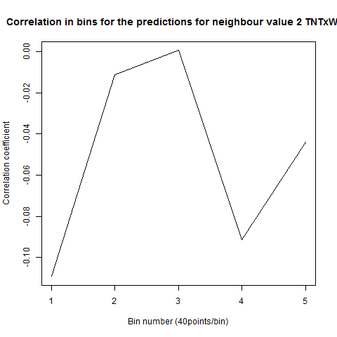
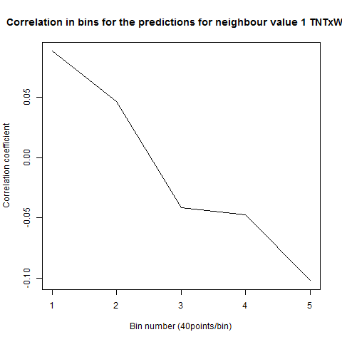
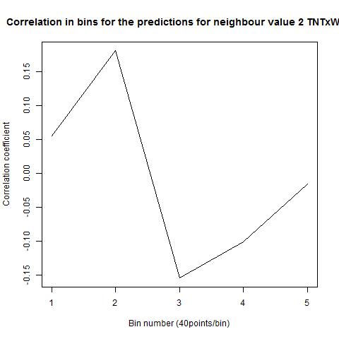
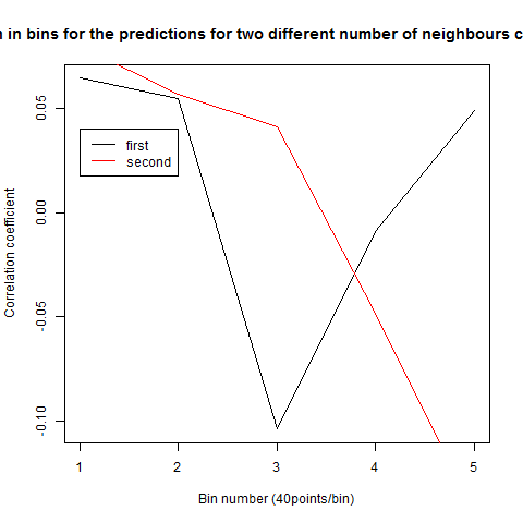
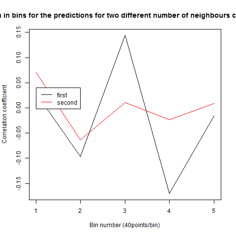
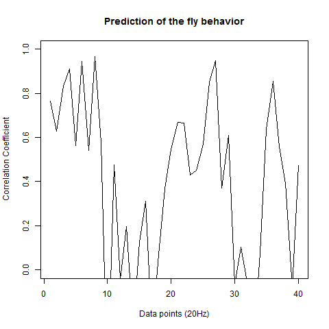
To see if there is an exponential decay in the prediction of the fly traces we did correlations of bins of 40 data points. We have 4 graphs (the last one merged) which consist of predictions at two different points with two different number of neighbours used for the prediction. So we have for each group sucesively: prediction at the first prediction point with the first number of neigbours, then the same with different number of neighbours. The last two are two different numbers of neighbours for the second prediction point. In the order: c105;;c232>TNT, TNTxWTB, c105;;c232xWTB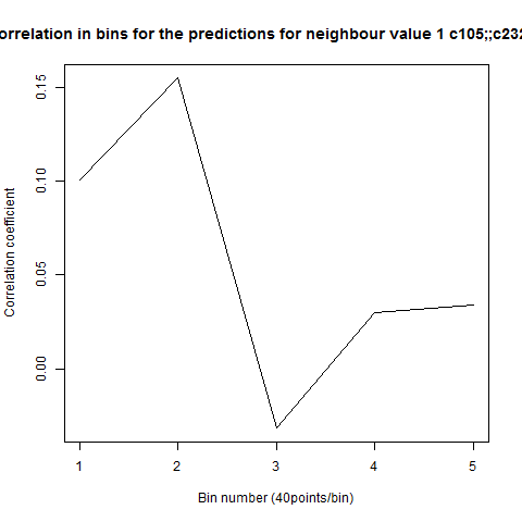
Category: R code, Spontaneous Behavior, strokelitude, WingStroke | No Comments
Nonlinear signature of Drosophila in Strokelitude
on Monday, March 14th, 2016 1:48 | by Christian Rohrsen
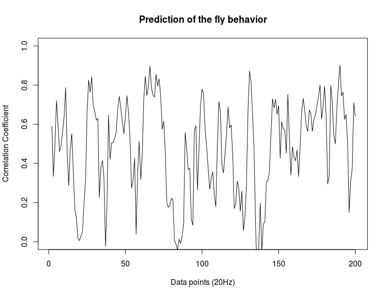
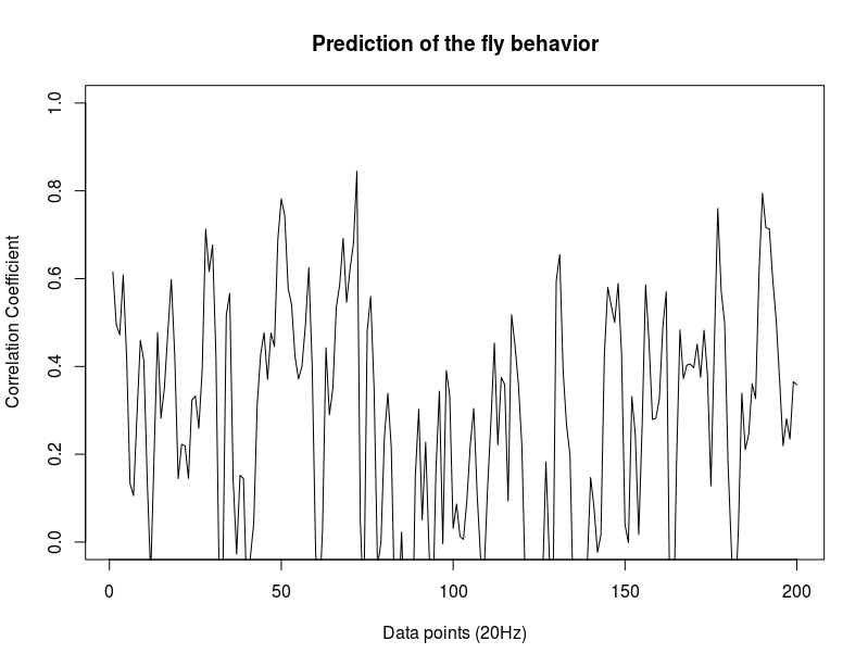
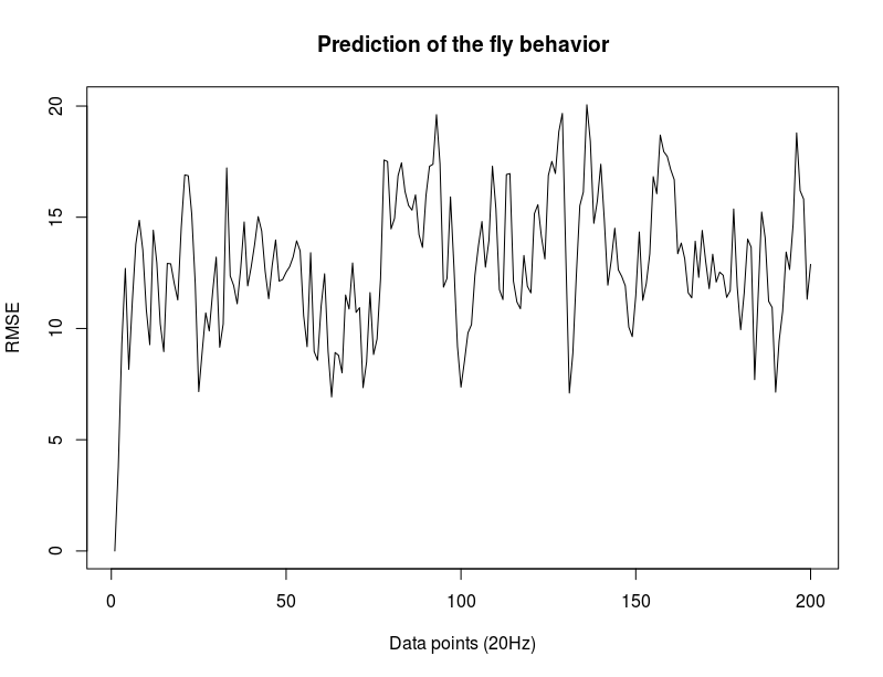
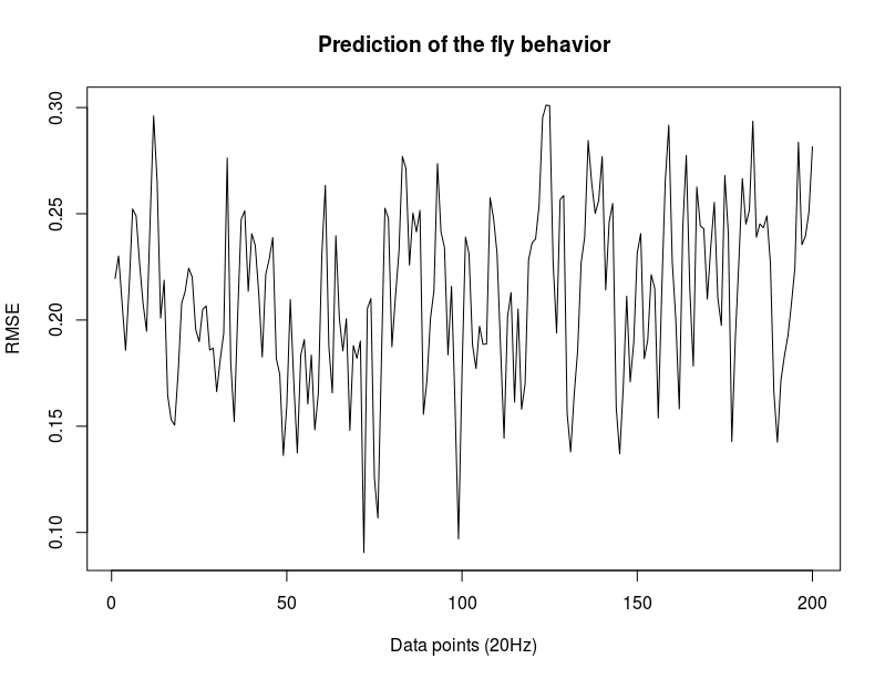
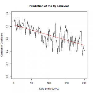
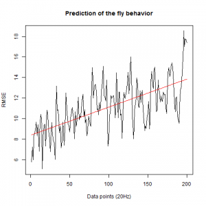
This is now the results from trying to predict the fly behavior doing ensembles of two predictions for the next 200 data points at two different points of the traces.
c105;;c232>TNT:
WTBxTNT: 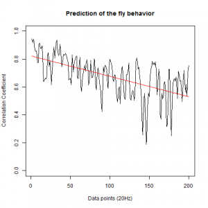
WTBxc105;;c232: 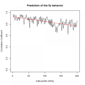
From what we see here, there is no “flattening” in the prediction of the fly when the neurons under c105 and c232 are targeted by TNT. This is done with around 14/15 flies for each group with two predictions in each ensemble of the two starting points. That makes a total of 15flies x 3 groups x 2 starting points for prediction x 2 predictions per ensemble = 180 prediction traces. Now I´m trying to calculate it by making correlations of bins in the prediction-observed for the same fly
Category: R code, Spontaneous Behavior, strokelitude, WingStroke | No Comments
Modelling the T-maze screen
on Monday, March 14th, 2016 1:35 | by Christian Rohrsen
This is the markdown showing the protocol and results of the modelling for the choice in the T-maze. This is for calculating valence. Nevertheless, this needs to be confirmed with the results of more lines, it could be that it is overfitted, I would like to do in addition cross-validation. I´m actually doing crosses and finding new lines to have more lines to test.
Category: neuronal activation, Operant learning, Optogenetics, R code | 1 Comment
Fly behavior prediction in the platform
on Monday, February 15th, 2016 2:25 | by Christian Rohrsen
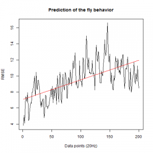
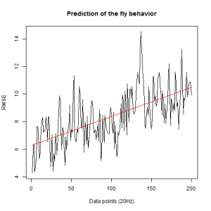
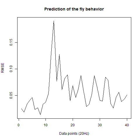
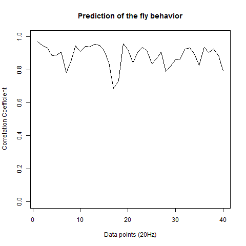
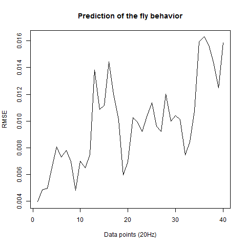
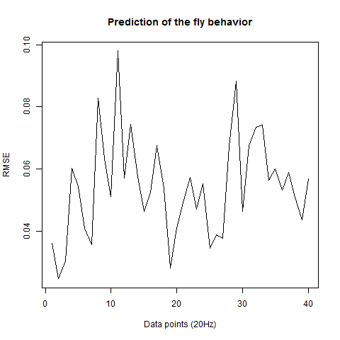
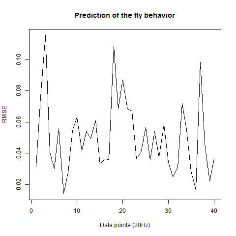
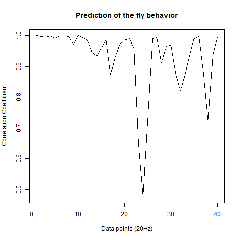
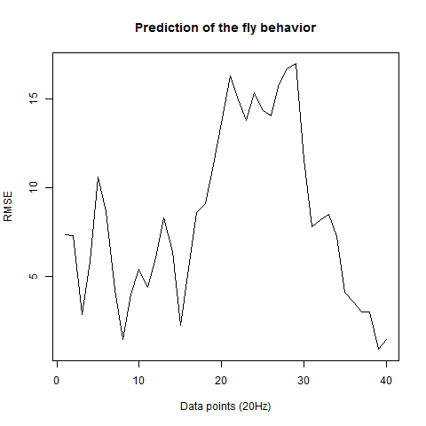
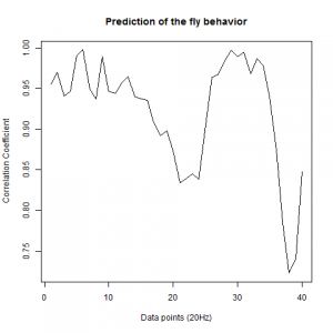
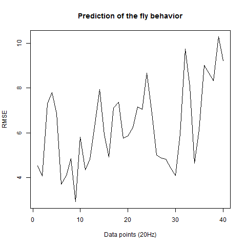
This is the prediction analysis of flies in the platform under a 20min experiment under dark conditions. The number of experiments change drastically among groups because of technical problems: WTBxTNT is 4, WTBxc105;;c232 is 22, for the experimental line is 6 (c105;;c232>TNT), for the platform without flies is 10. I show the root mean squares and the correlation coefficient for each group.
This is the experimental group: c105;;c232>TNT.
The group without flies on the platform. I expect here to get a very good predictability overall:
WTBxc105;;c232 group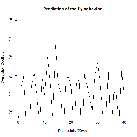
 WTBxUAS-TNT
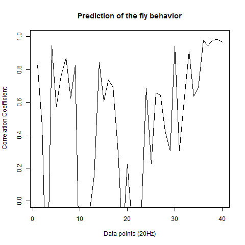
Category: R code, Spontaneous Behavior, strokelitude | No Comments
First tests of fly prediction under a mean of the flies on single data points
on Monday, February 8th, 2016 12:11 | by Christian Rohrsen
These were done the week before last one but I could not upload it last time, so here are they. These are the results for predicting 4-5 flies of each group. Just one prediction from the middle of the time series for the 40 data points ahead in the future. First group is c105;;c232>TNT.
This is c105;;c232 x WTB
This is UAS-TNT x WTB 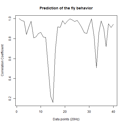
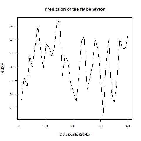
As I saw that the graph had so much zig-zag I told Pablo to make a bigger number of tested flies and this is what he is presenting today.
In addition I did analyze other parameters which are all saved under a PDF file below (Strokelitude). This contains some parameters with doubtfull processing which I still don´t trust so I have to find a better way for the calculation of it.
Category: R code, Spontaneous Behavior, strokelitude | No Comments