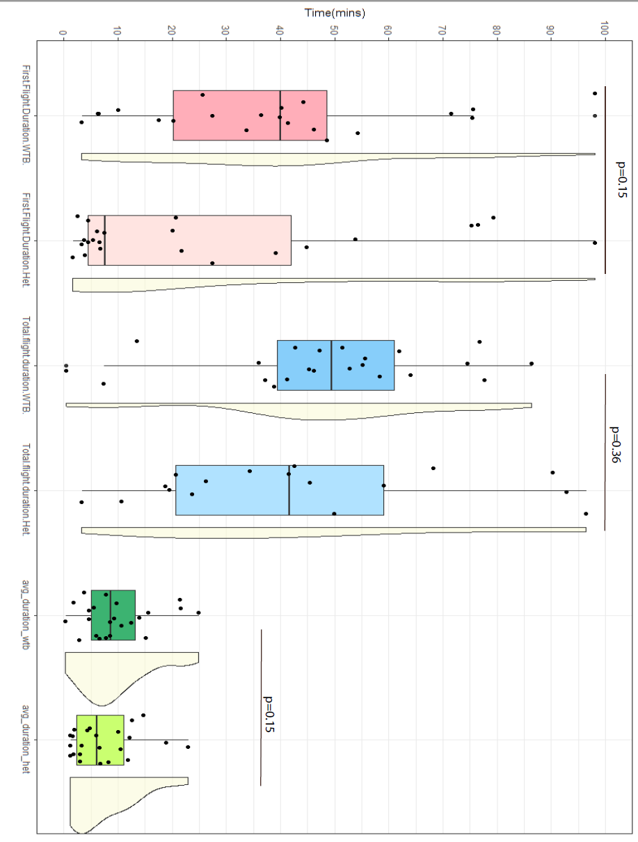
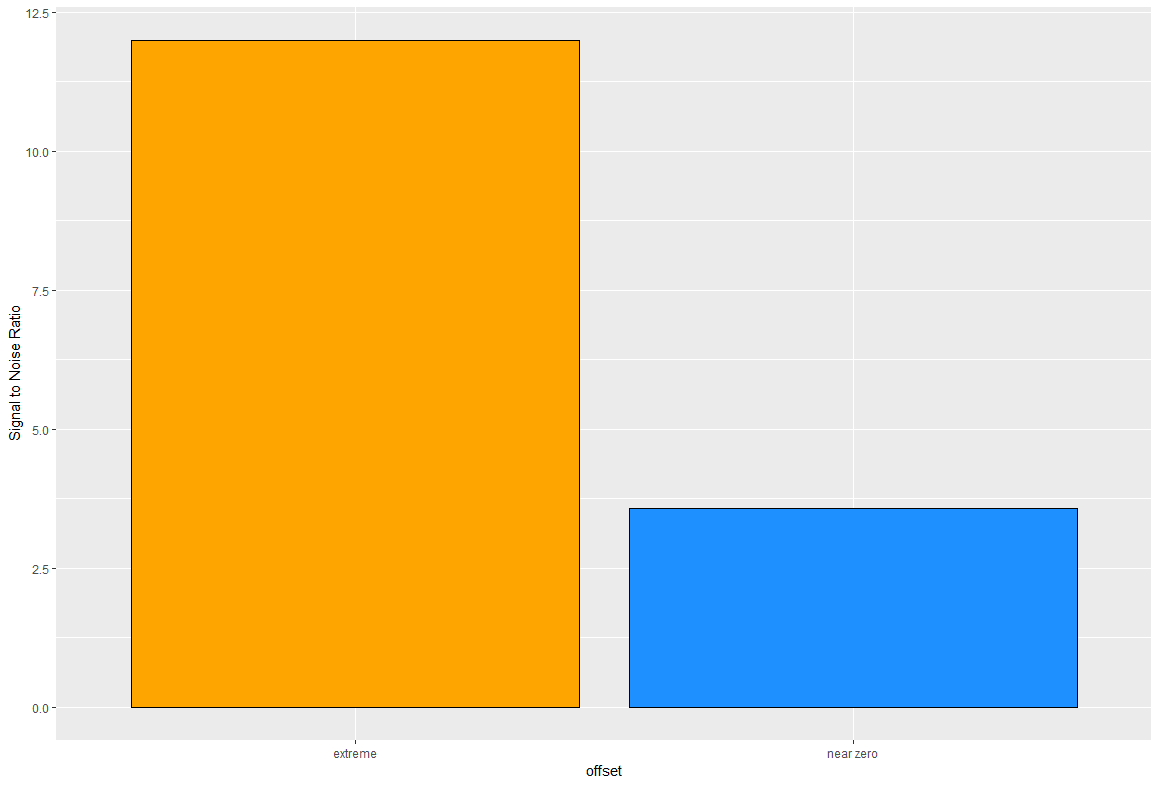
Signal to Noise Ratio, flight Performance (Het)
on Monday, October 8th, 2018 2:02 | by Saloni Rose
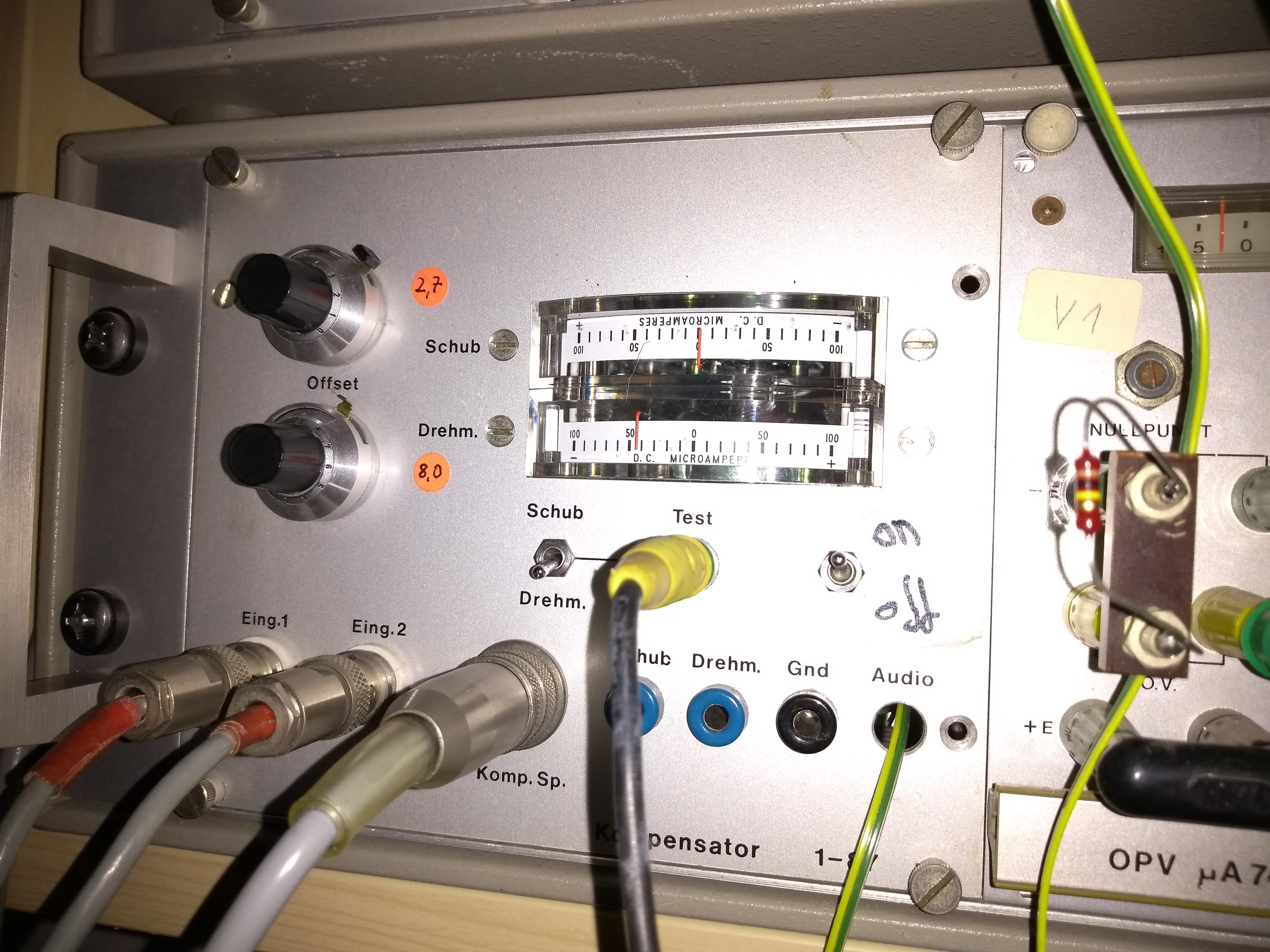
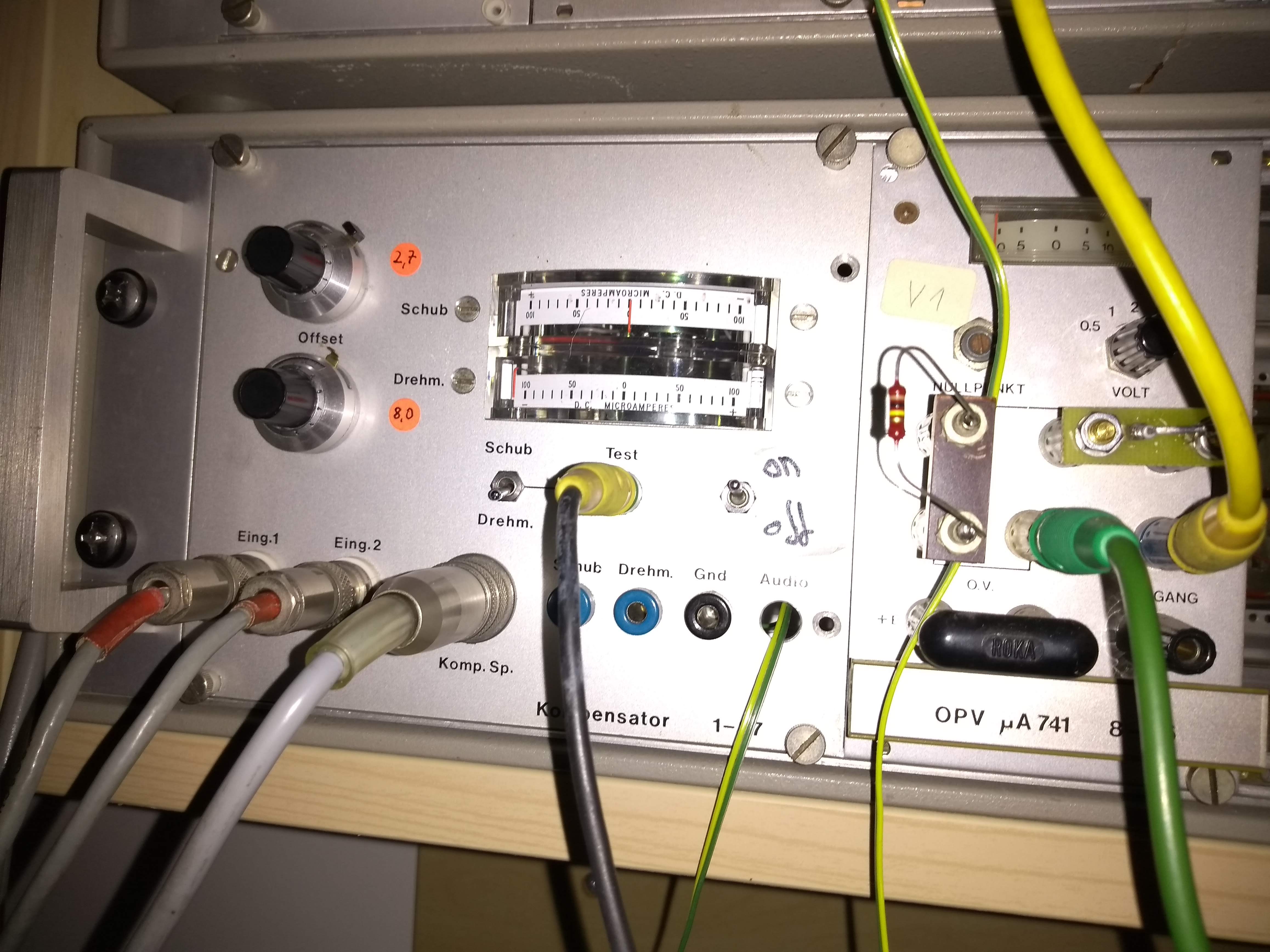
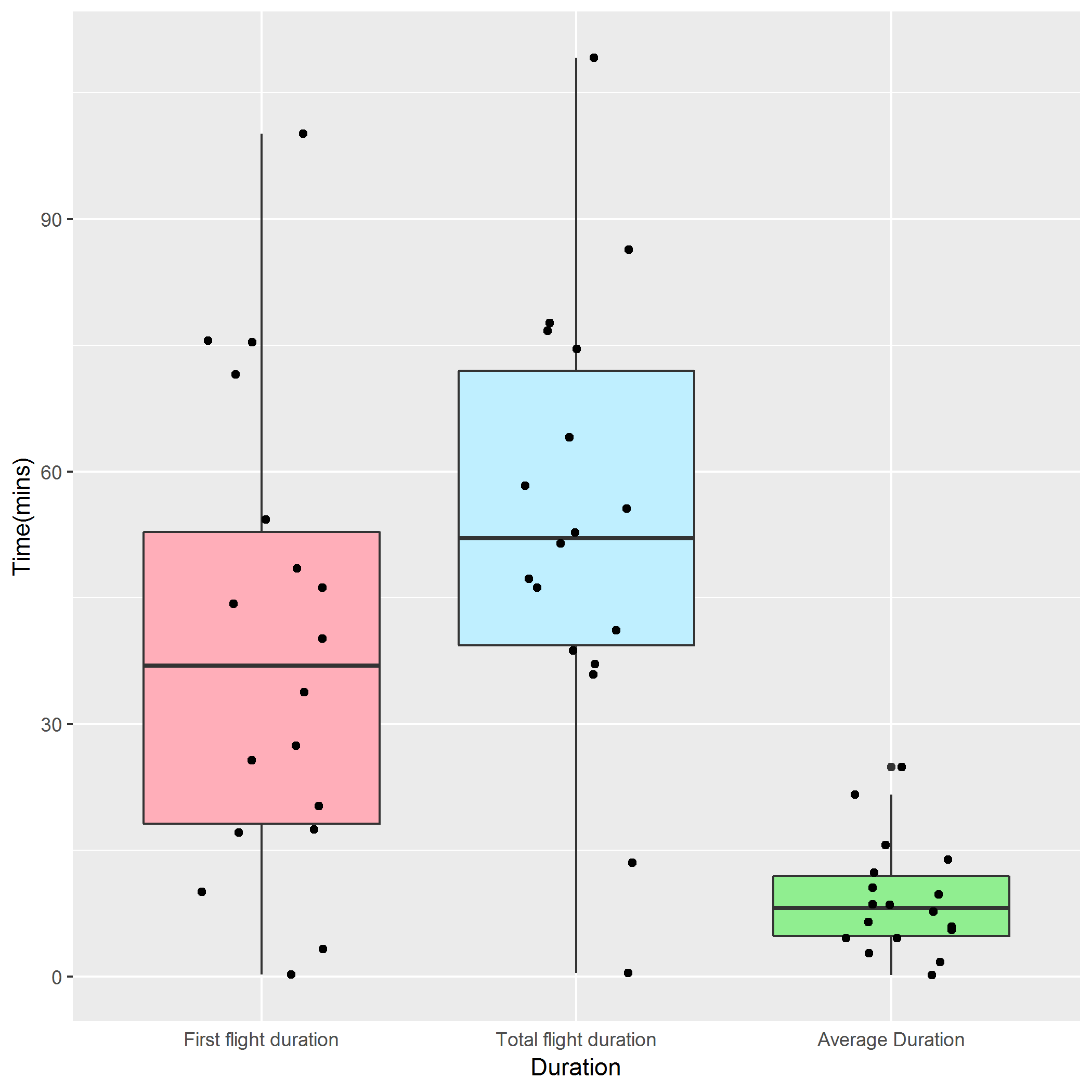
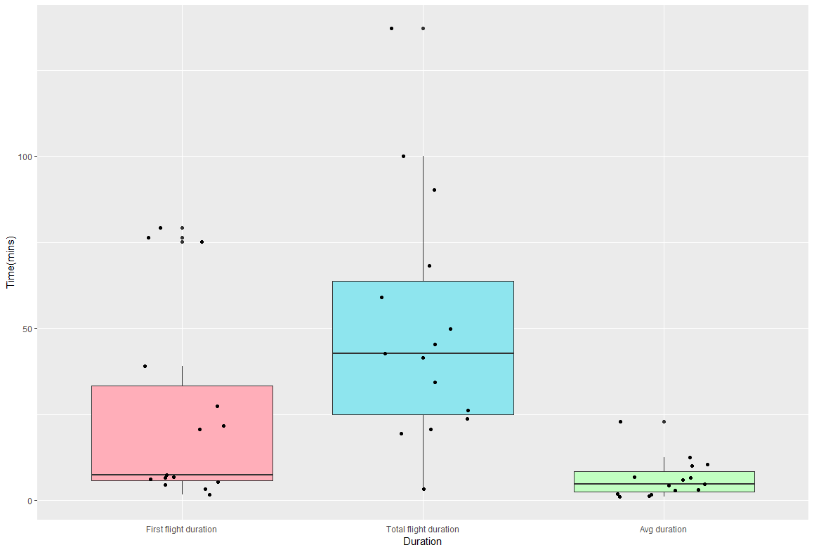
Torque trace flies
https://drive.google.com/open?id=1utjuIrgQogT2lrRMl32VNdaBhsV_Ii5d

Category: Uncategorized | No Comments
Bits & Pretzels 2018
on Monday, October 8th, 2018 10:57 | by Max von der Linde
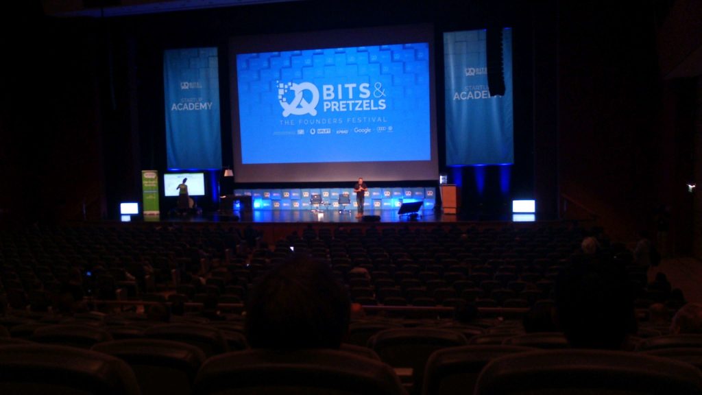
The fair took place from 30th September – 2nd Oktober (Sunday to Tuesday). I attended at Monday and Tuesday. The first two days were located at the Messegelände Ost Munich while for the last day the “Schottenhammel” Tent at the Oktoberfest had been reserved.

Monday:
Visit of the “Corporate Stage” which showcased Interviews:
– The guest came from Adidias but worked independently first- before Adidas she used to make statistical interpretations on her own and present them to companies-> inefficient, it makes more sence to first inquire what the company is interested in- more and more Big Data with high tech factories- example of practical use of statistics: spike in sales as Kanye West fashioned a certain shoe
AI


2. Divide and conquer debugging: break code up smaller and smaller until you reach the line with the problem





Category: Uncategorized | No Comments
Program testing & Histogram Comparison
on Monday, October 8th, 2018 9:20 | by Max von der Linde
Is the program doing its job? Manual stimulation of the platform:
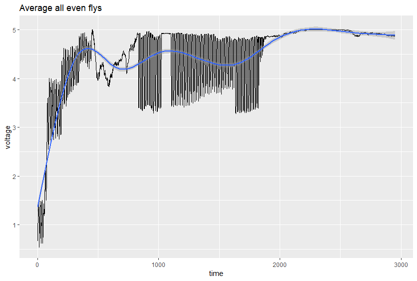
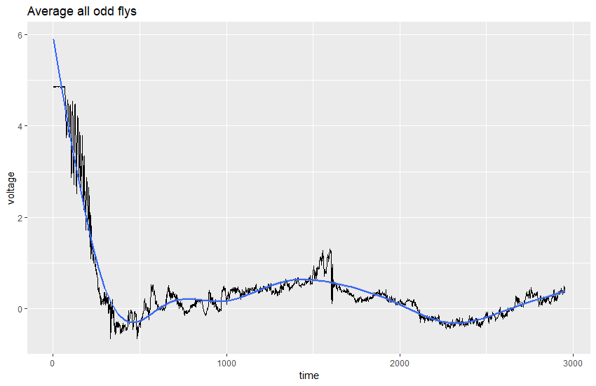
-> yes it is
Histograms
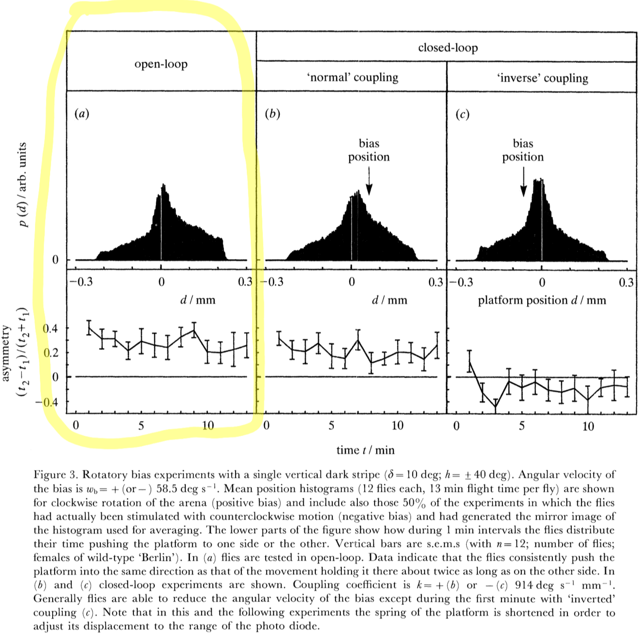
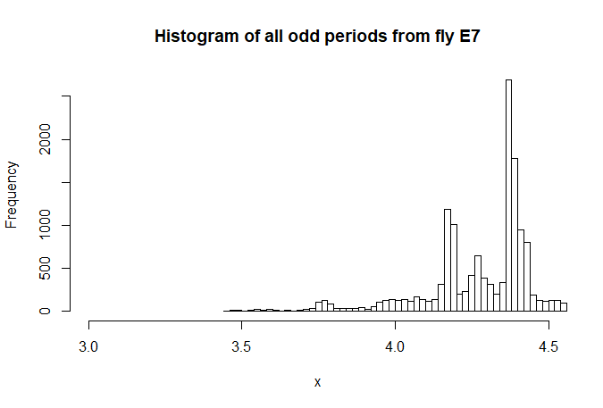
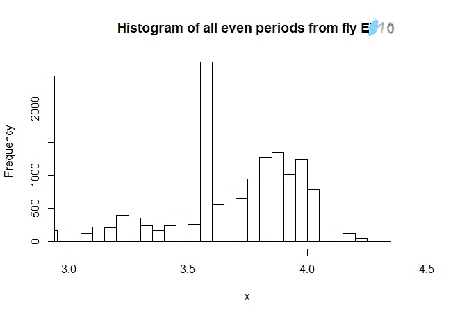
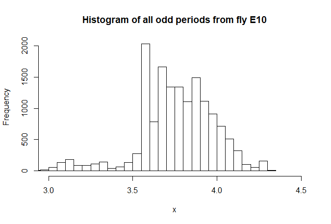
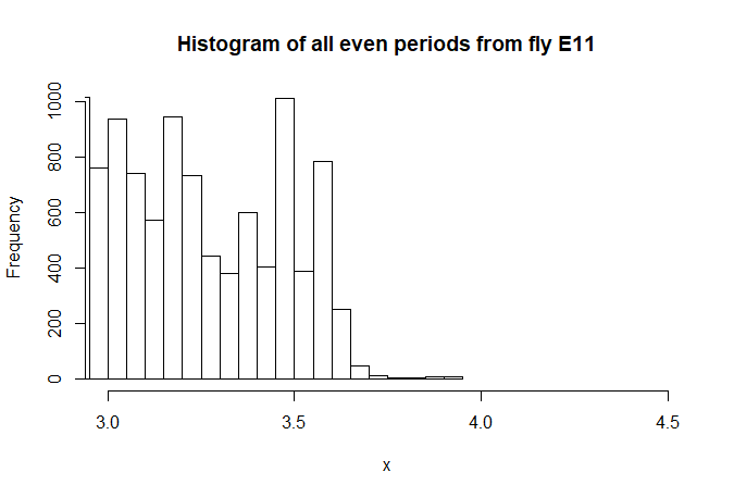
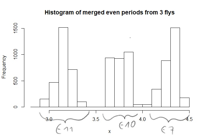
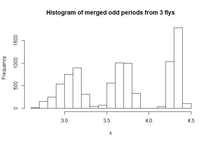
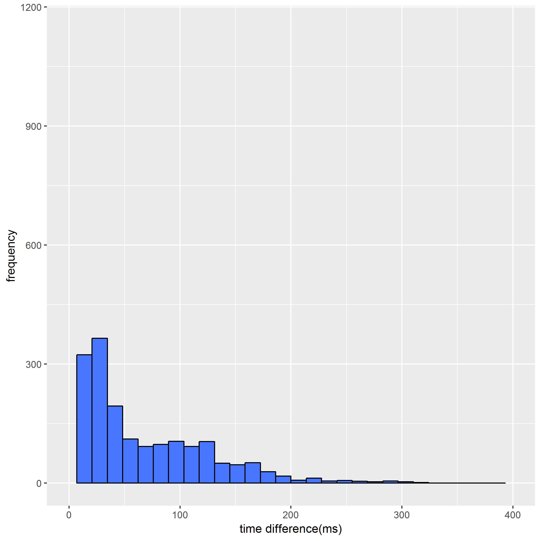
Why frequency histograms? I want to compare my data to the data from “Can a fly ride a bicycle?” (Wolf 1992):
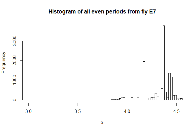
example fly E7:

example E10:
example E11
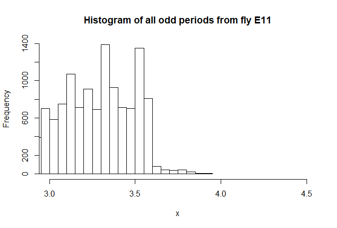
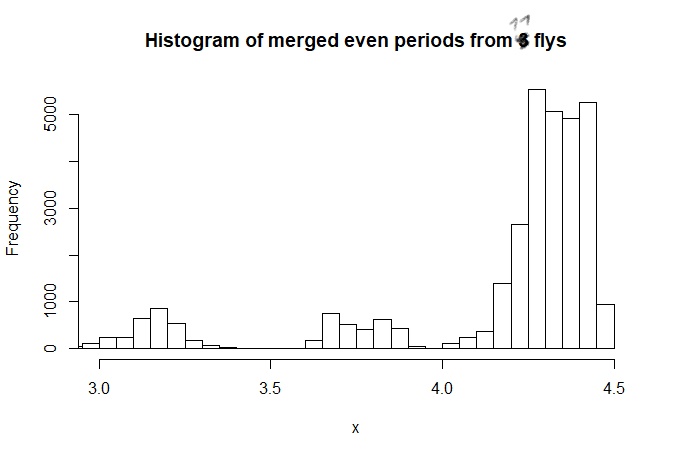
Histogram of 3 flys (periods of idividual flys have been merged -> one odd and one even period per fly):
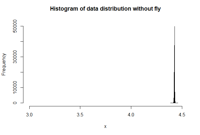
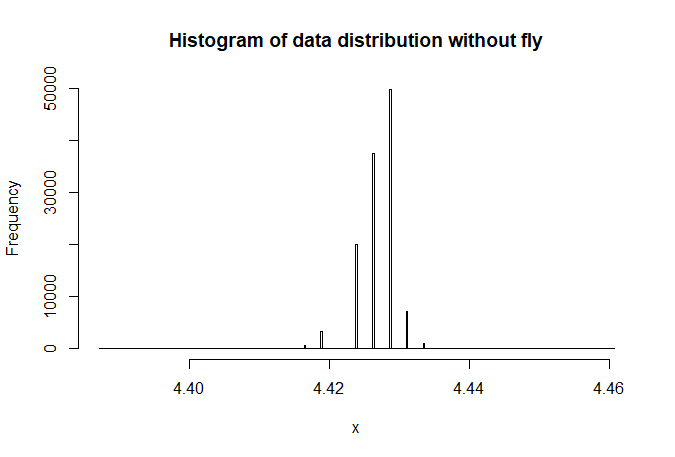
Histogram of platform without fly:
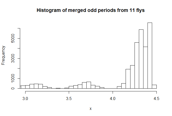
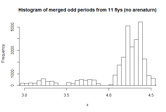
Histogram of 11 flys (periods of idividual flys have been merged -> one odd and one even period per fly):
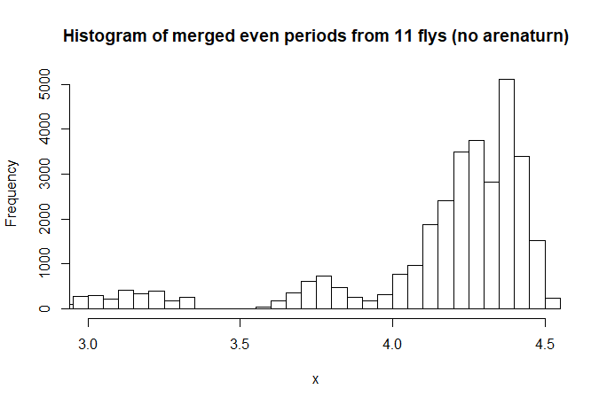
Histogram of 11 flys (no arenaturn):
Fly 3 (discussion model)
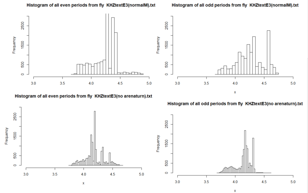
All Histograms of different tests for fly 3
-> merging makes little sence if the distribution is completely different areas for each fly!
Category: Uncategorized | No Comments
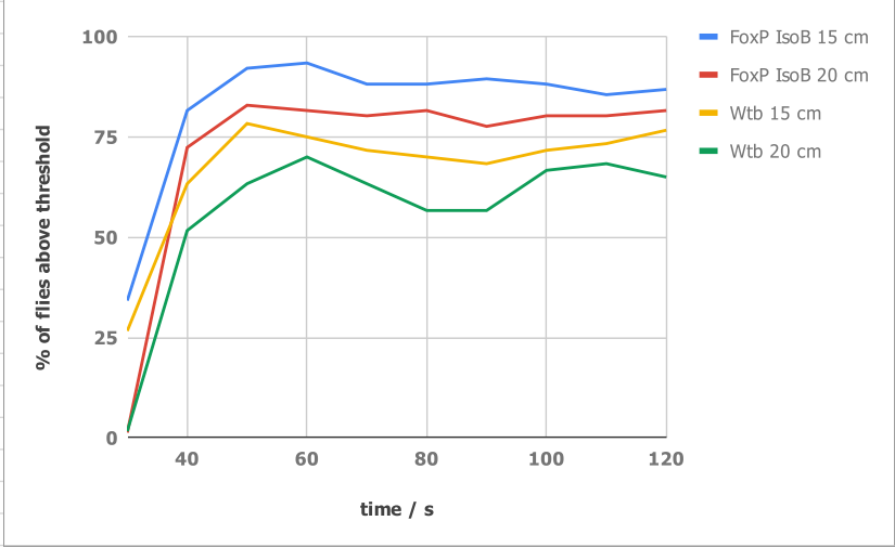
FoxP flight simulator
on Monday, October 1st, 2018 2:55 | by Anders Eriksson
Category: Uncategorized | No Comments
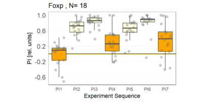
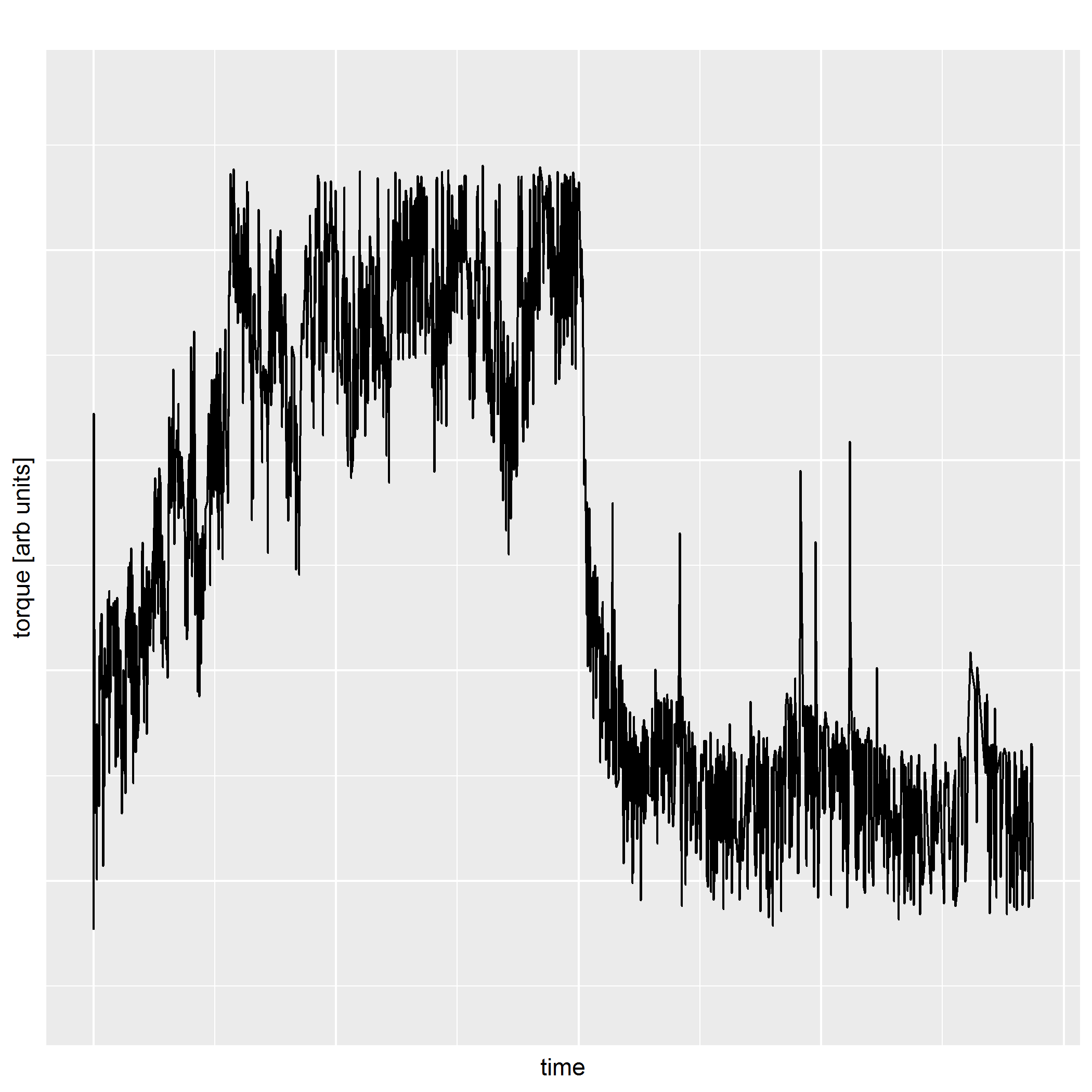
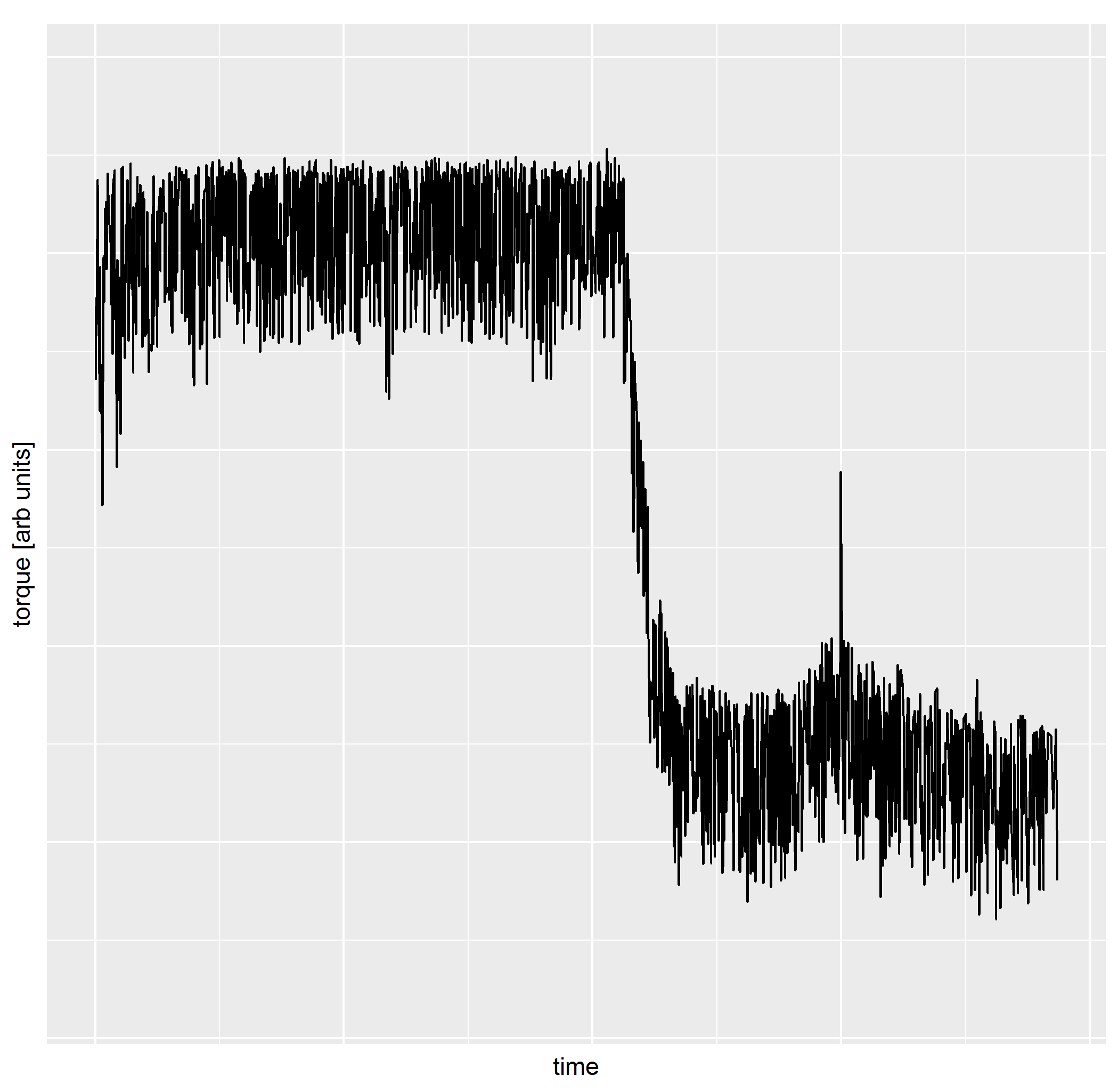
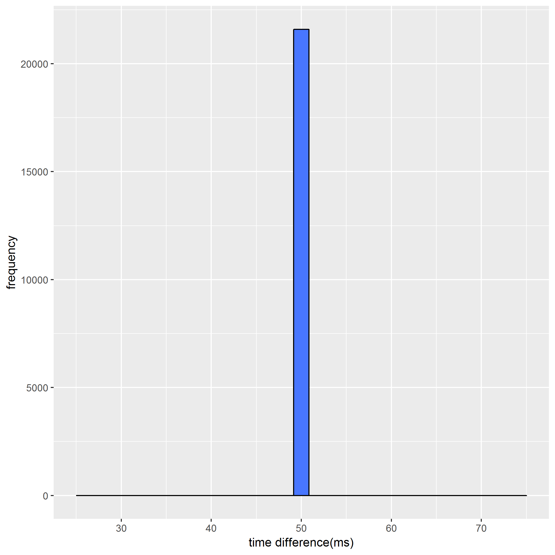
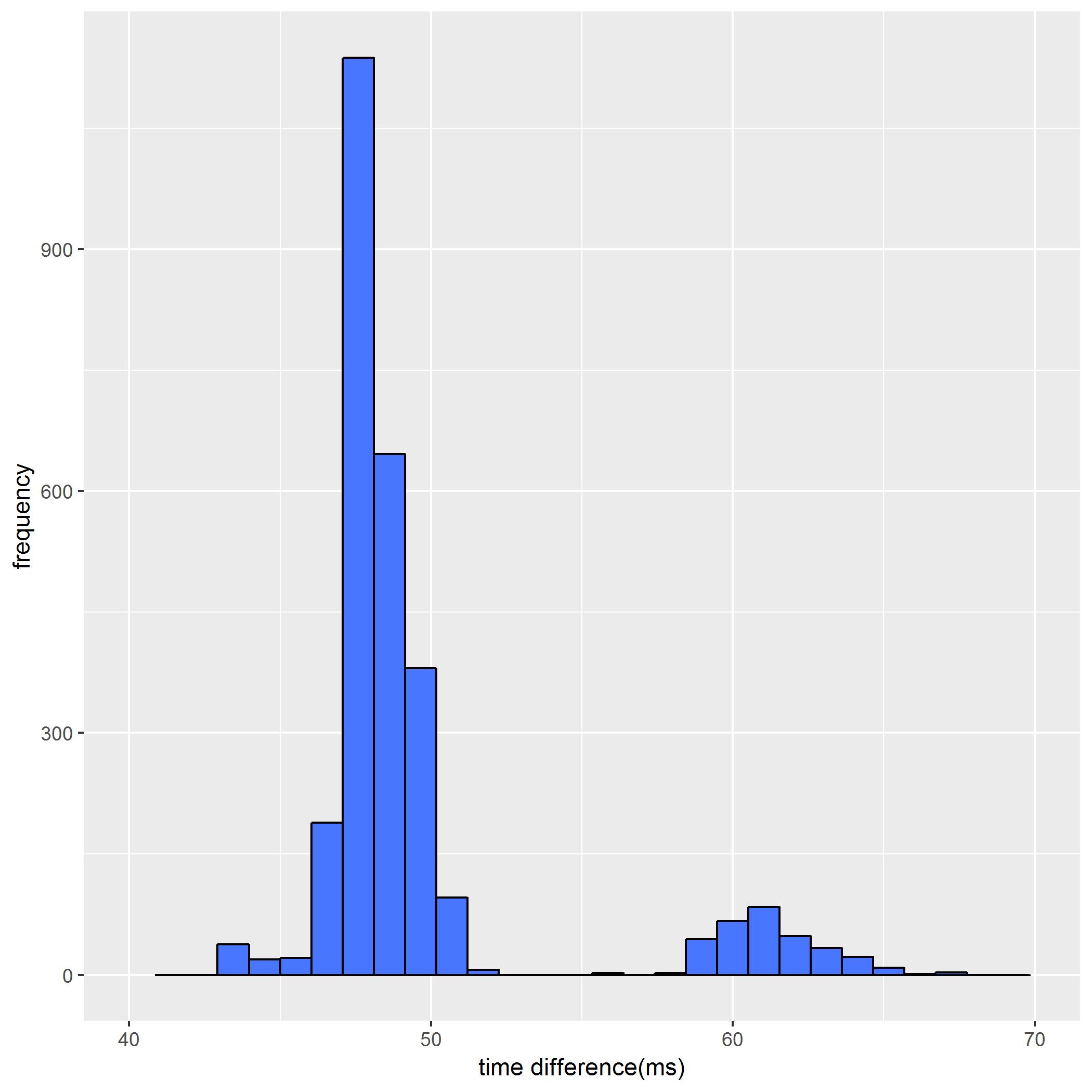
Flight Performance data, Optomotor response
on Monday, October 1st, 2018 12:41 | by Saloni Rose
Category: Uncategorized | No Comments
Beta results from first test drive OptoMoto
on Monday, September 24th, 2018 1:56 | by Max von der Linde
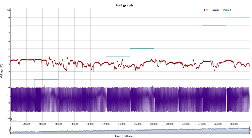
The different stages of data processing:
1. single fly dyplot with all data present
E11(normalF)
2. Plot of all the even / odd periods of one fly
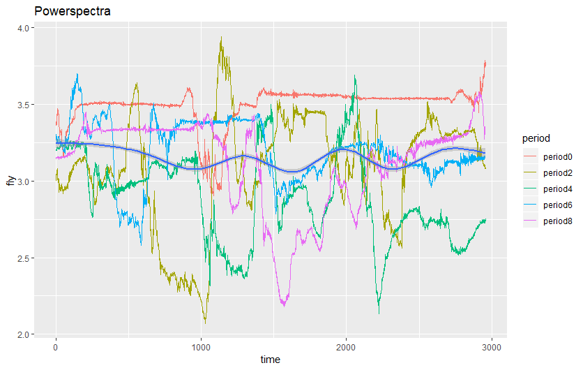
E11(normalF)even_period_plot
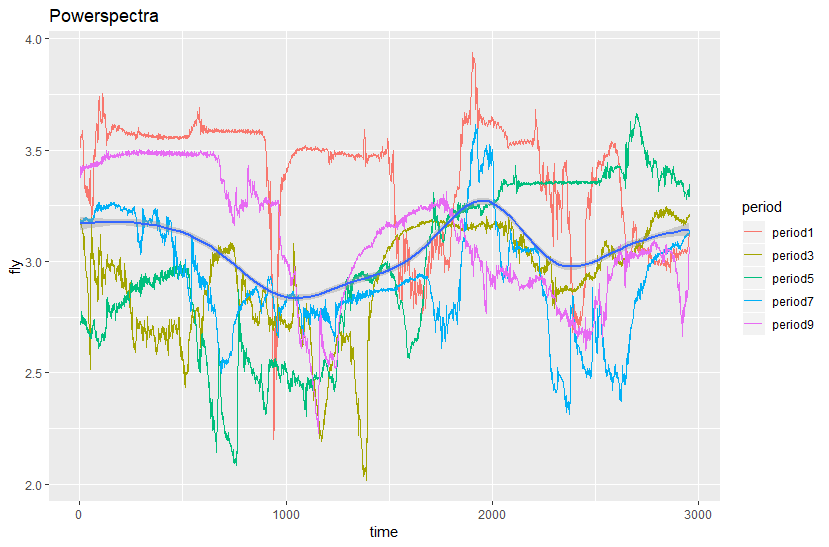
E11(normalF)odd_period_plot
3. Plot of all even / odd Periods of one fly merged
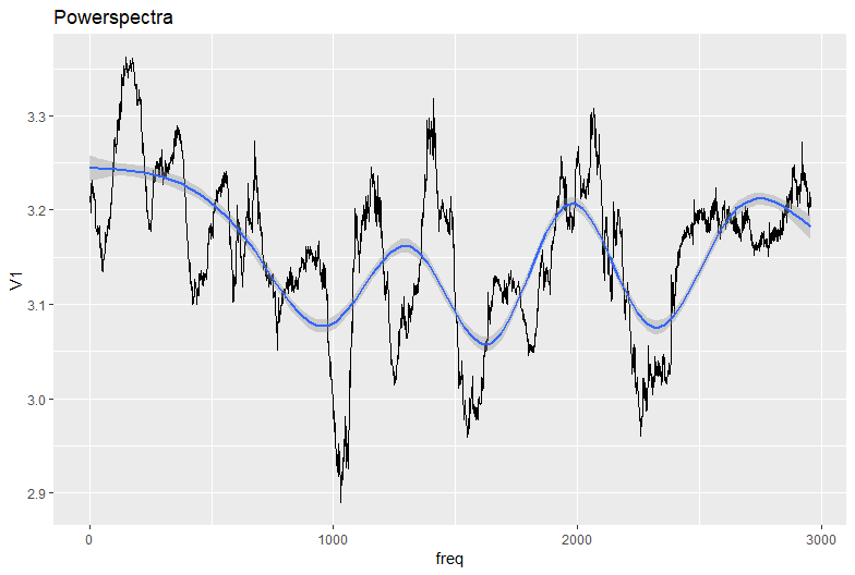
E11(normalF)even_merged_plot
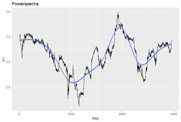
E11(normalF)odd_merged_plot
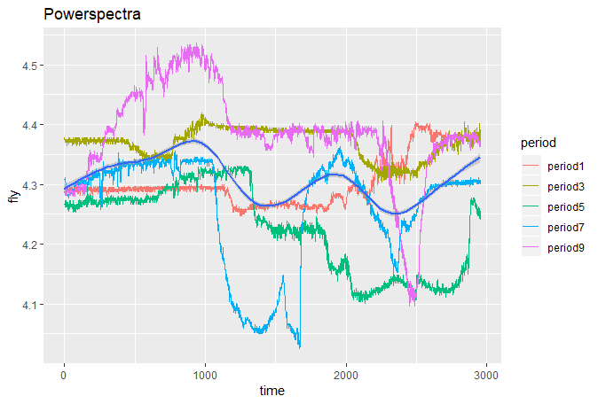
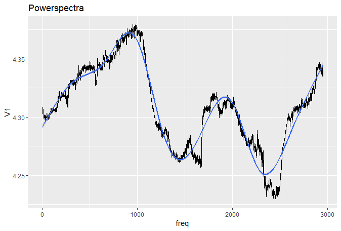
4. Plot of the even/odd periods from all tested flys
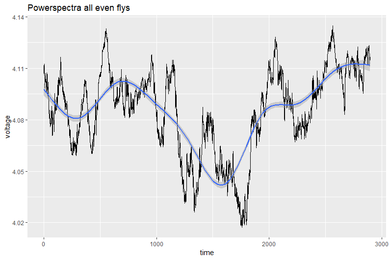
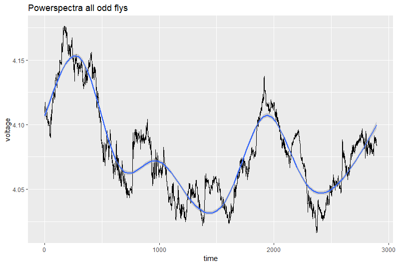
Another example (first fly tested):
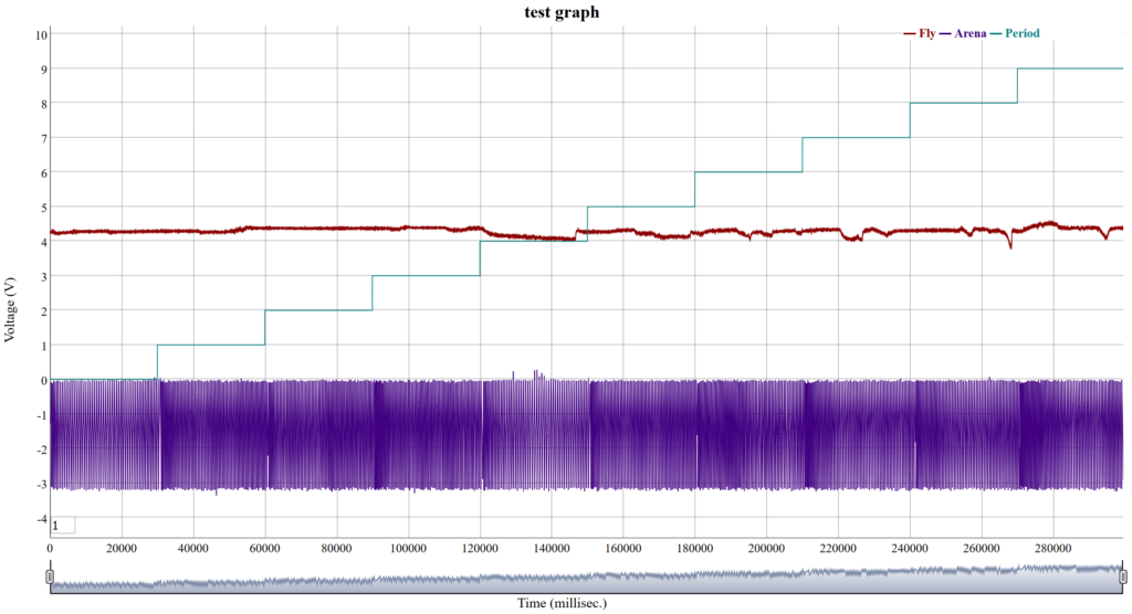
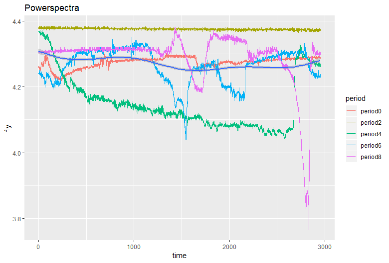
E1(normalF)period_plot
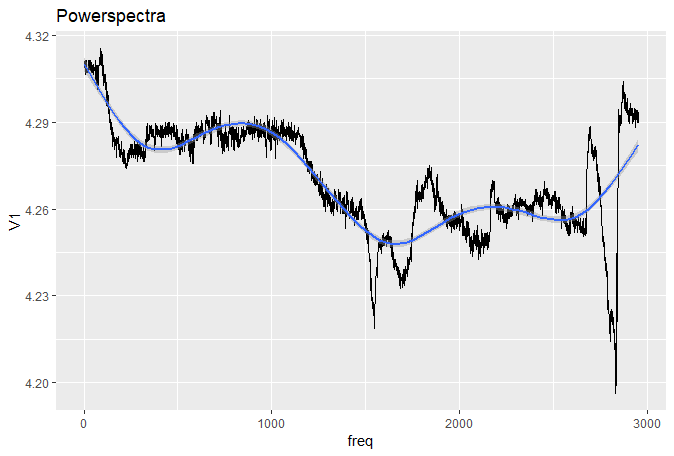
even_merged
Category: Uncategorized | No Comments
Datahandling OptoMotorics
on Monday, September 17th, 2018 12:31 | by Max von der Linde
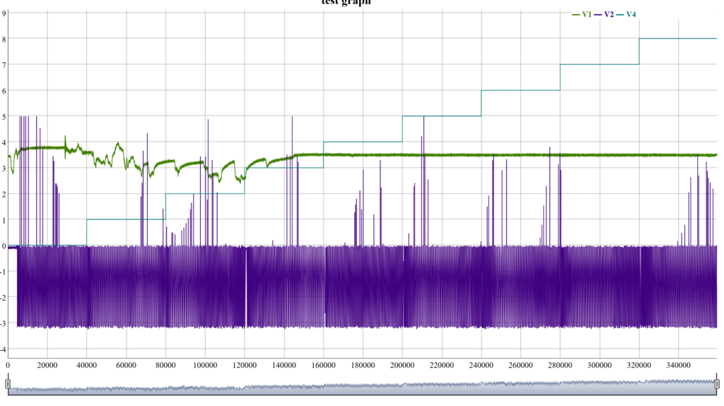
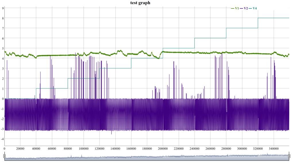
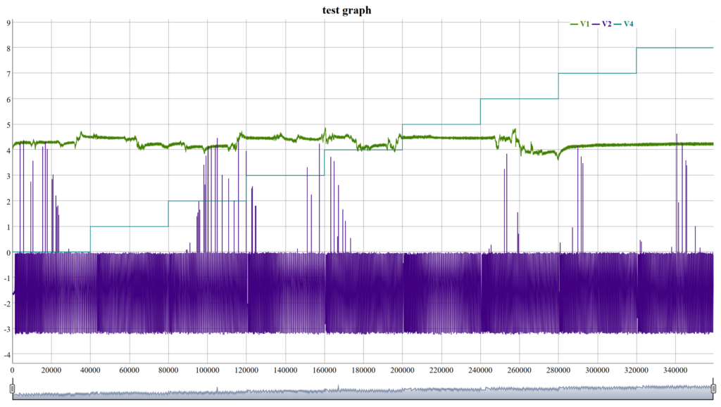
Table with the generated fly test data:
| Test | Description | Average right | Average left | Differece | general |
| Ex4 | normal | 4.55382 | 4.624879 | 0.071059 | 4.5893495 |
| Ex4 | repositioned | 4.562121 | 4.579682 | 0.017561 | 4.5709015 |
| Ex5 | normal | 4.273299 | 4.434383 | 0.161084 | 4.353841 |
| Ex5 | repositioned | 4.562121 | 4.579682 | 0.1610834 | 4.5709015 |
| Ex6 | normal | 3.535669 | 3.587334 | 0.051665 | 3.5615015 |
| Ex7 | no arena | 3.349097 | 3.337588 | -0.0115097 | 3.343343 |
| Ex8 | bad fly | 3.42903 | 3.394603 | -0.034427 | 3.411816 |
| Ex9 | no arena | 4.391139 | 4.363279 | -0.0278599 | 4.377209 |
| Ex9 | normal | 4.404213 | 4.456195 | 0.05198185 | 4.430204 |
| Ex10 | no arena | 4.259827 | 4.195971 | -0.0638559 | 4.227899 |
| Ex10 | normal | 4.243121 | 4.360124 | 0.1170035 | 4.301622 |
Ex8:
Ex9:
Ex10:
Category: Uncategorized | No Comments
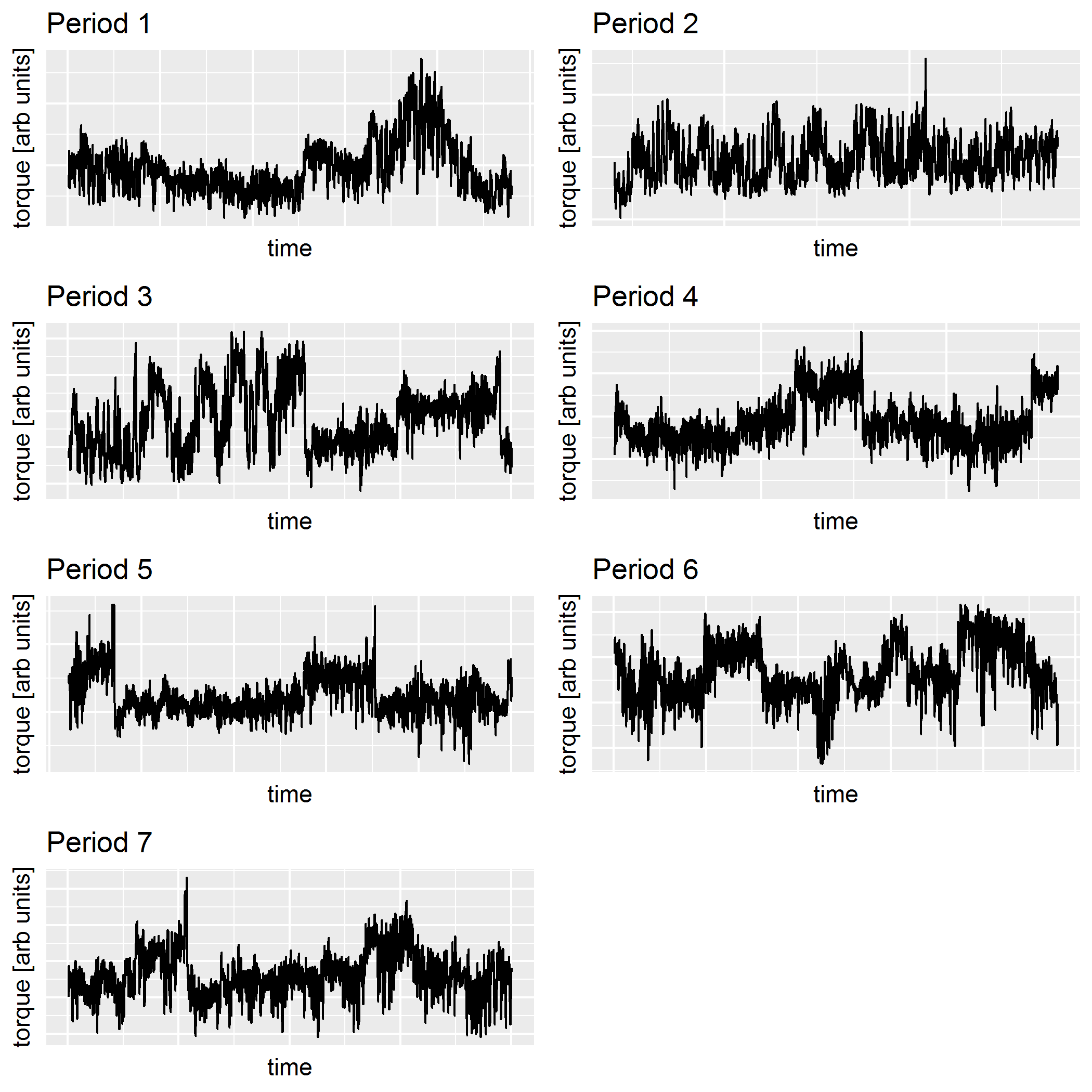
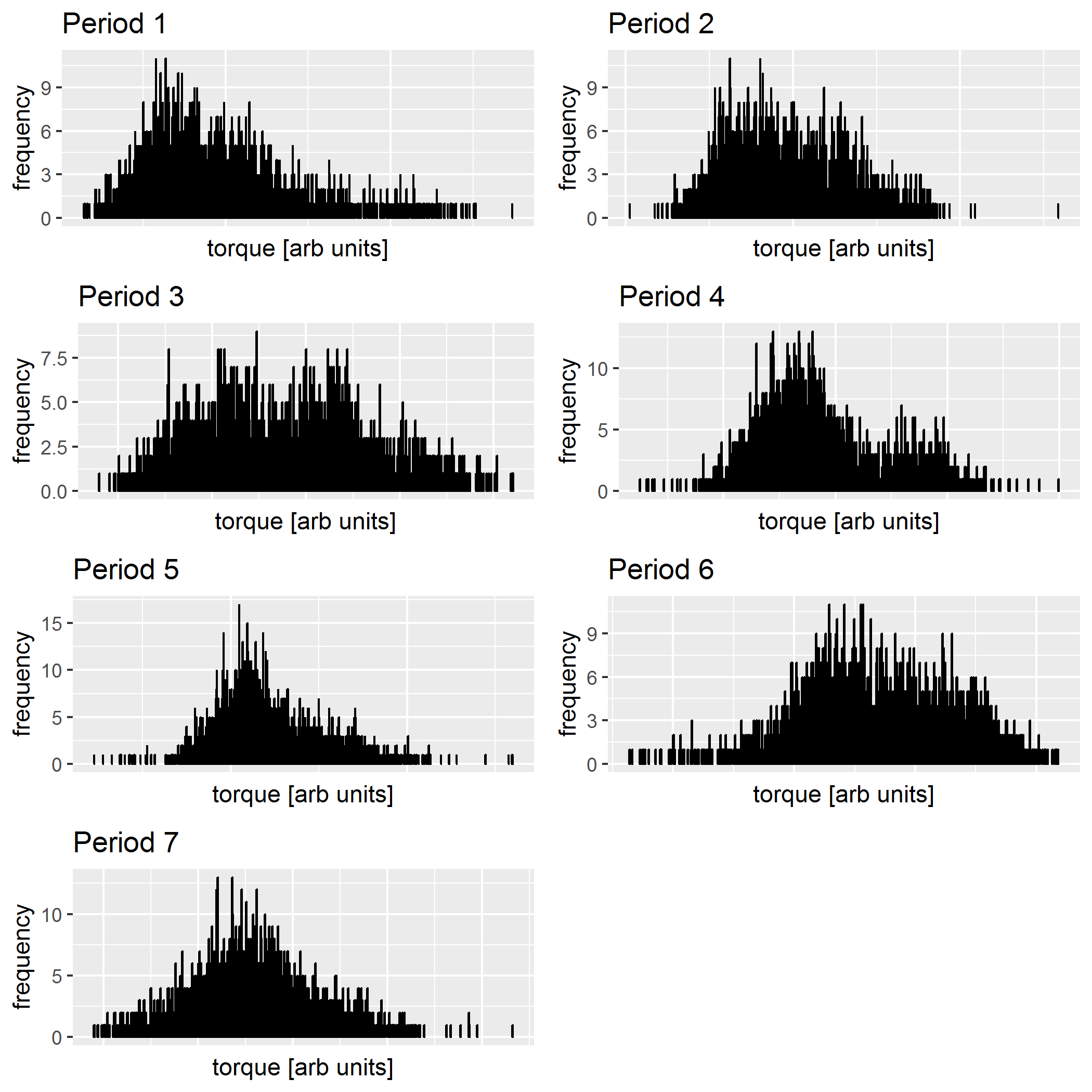
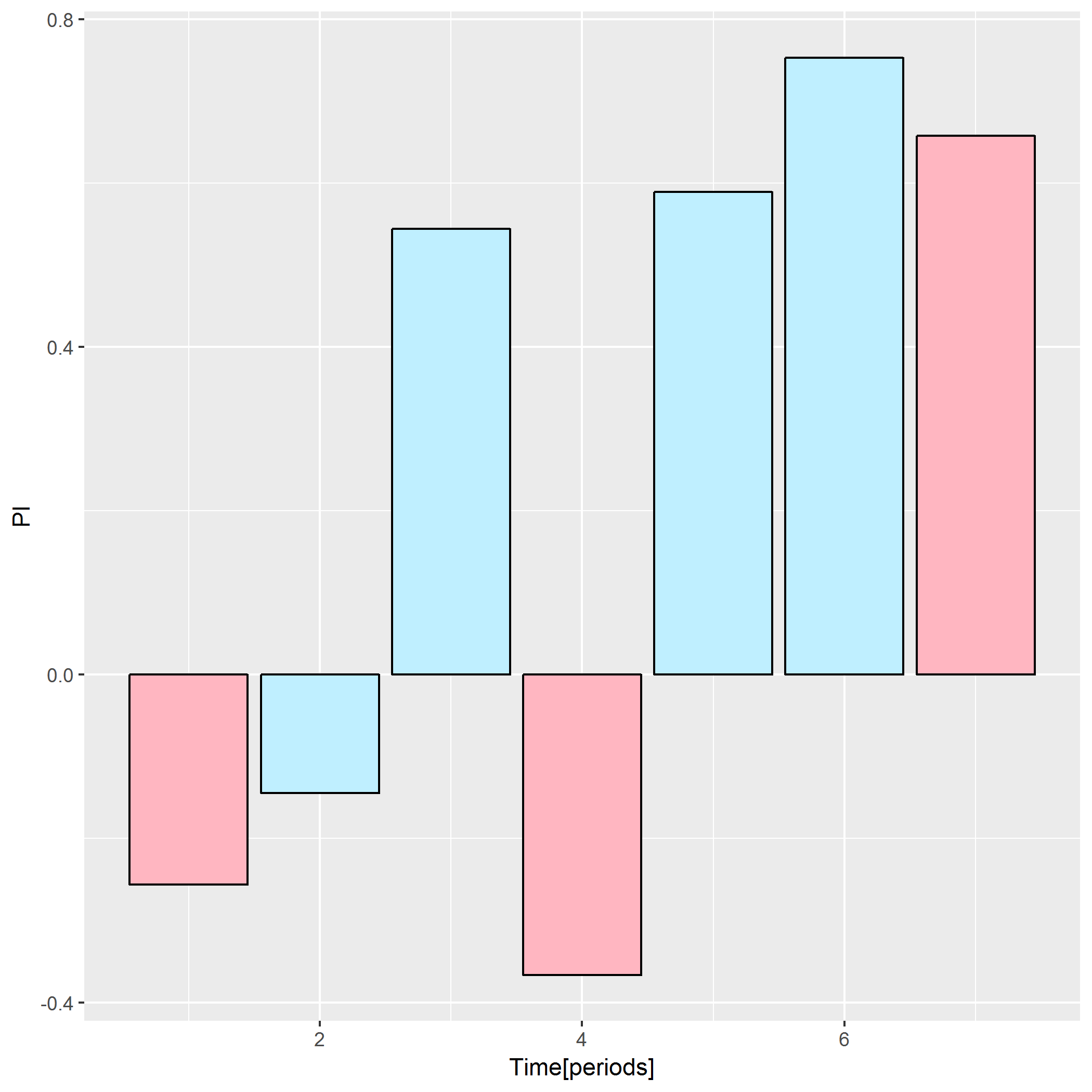
First Dataset From OptMoto Experiment
on Monday, September 10th, 2018 12:07 | by Max von der Linde
Text data file with all the rawdata generated by my new programme: Rawdata OptMoto
R programme which generates the plot:
library(dygraphs)
rawdata <- read.csv(“KHZtext.txt”, header = FALSE, sep = ” “)
flydata <- rawdata[c(3, 1)]
#dygraph(flydata) %>% dyRangeSelector()
arenadata <- rawdata[c(3, 2)]
rawdata <- rawdata[c(3, 1, 2)]
dygraph(rawdata, main = “test graph”) %>%
dyRangeSelector()
# dySeries(“V1”, name = “fly”) %>%
# dySeries(“V2”, name = “arena”) %>%
# dyAxis(“y”, label = “Voltage (V)”) %>%
#
Category: Uncategorized | No Comments