Spontaneity: Measuring Wingstroke Amplitude with Strokelitude

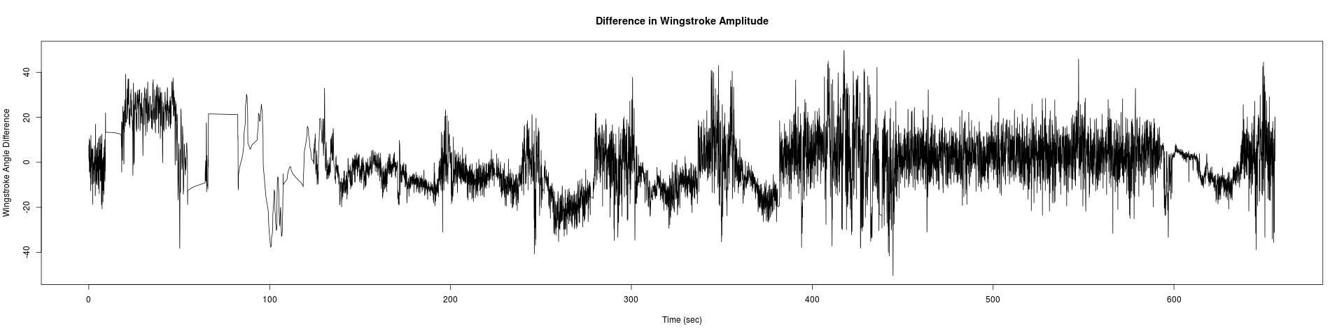
Those are the results of measuring the wingstroke amplitude with Strokelitude and “The ping pong ball machine”. And analysed with R studio and the scripts written by an student.

The results are not too good, comparing them with the result obtained in other experiments.

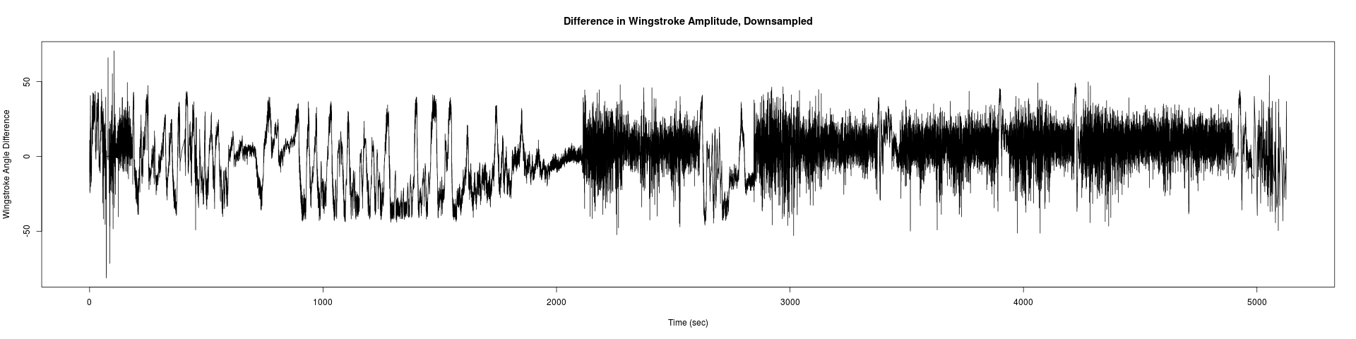
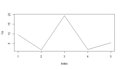
Two pictures of the trace down-sampled of my flies:

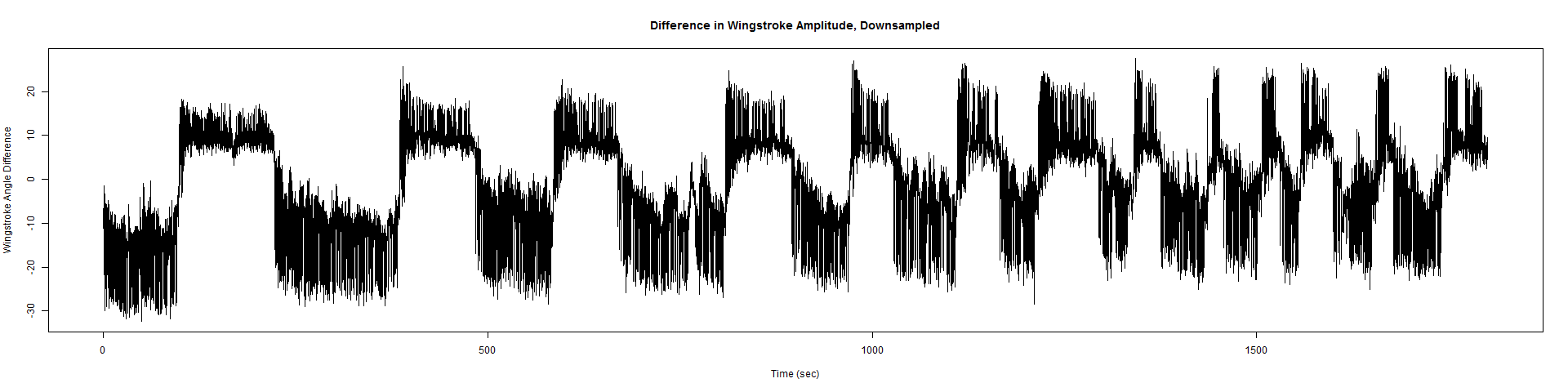
and in the next picture is how it should be plotted:

Installing fview and strokelitude

1. Install ubuntu, optimally the distribution precise pangolin (ubuntu 12.04 LTS) and get all relevant updates

2. Install fview

Using a terminal execute the following commands:
sudo gedit /etc/apt/sources.list
– at the end of that file, add the line deb http://debs.strawlab.org/ precise/
sudo apt-get update
sudo apt-get install camiface
sudo apt-get install python-motmot-fview
sudo apt-get install libhdf5-serial-1.8.4
sudo apt-get install hdf5-tools
sudo apt-get install python-tables=2.3.1-2ubuntu3
sudo apt-get install python-chaco
sudo apt-get install python-pylibusb
sudo apt-get install pyro
sudo apt-get install python-motmot-fastimage
sudo apt-get install python-motmot-realtimeimageanalysis
sudo apt-get install python-motmot-fviewexttrig

The installation of libhdf5-serial-1.8.4 might fail if there is already a newer library installed. Usually this should not be a problem, as long as the other commands work. To make sure, after executing all those commands you can run “sudo apt-get install -f” and see whether it shows you any conflicts. If there are no conflicts, the installation should have been successful. If there are conflicts, this command might be able to resolve them.
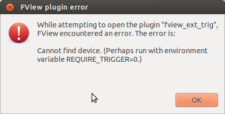
– test fview by executing the command fview (an error message will appear saying that no device was found. Ignore that.)
3. install strokelitude

sudo apt-get install python-strokelitude

– test fview again, now you should be able to start strokelitude under windows -> -=|strokelitude|=-

Measuring Wingstroke Amplitude with Strokelitude

The day before the measurement:
Glue the flies on hooks, put them into the single-fly valves and give them sugar and water to survive the night. Store them at the appropriate temperature

The day of the measurement:

1. Put the fly in position
Select a fly and put it in the clamp. Then put the clamp in the holder and position the ping-pong ball (or generally, the measurement environment) around the fly.
2. Set up the camera
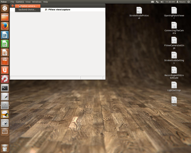
Start the computer and open fview (either by typing “fview” in a terminal or clicking the fview symbol on the launcher). Close the error message that fview produces.

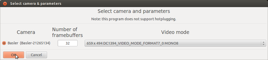
Then initialize the camera (click “Camera” -> “Initialize Camera” and click OK in the window that pops up).

If fview does not list your camera as a candidate for initialization, you may have to configure your connection to the camera. Go to the Ubuntu System Settings and select “Networks”. Here, select the connection via which the camera should be connected to your computer. Open “Options” and “IPv4 Settings” and set “Method” to “Local Only”.

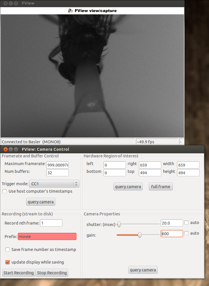
In case the image you get after initialization is very small (only a tiny square in the upper left corner of the fview window), change to a different desktop and back. This should usually solve the issue.

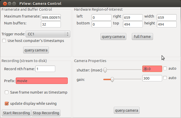
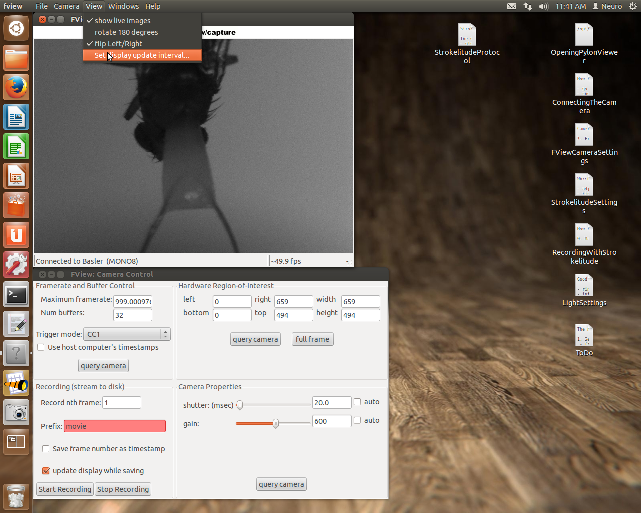
Open the camera settings (via “Windows” -> “Camera Controls”) and put the “shutter(msec)” to 20. During the actual recording the shutter should be at 10 msec to reach a sampling rate of ~100Hz, but for the setup it is more convenient to have it at 20 or 30. Now adjust the gain until you can see something on the picture. Then use the micro-manipulator to move the camera until you have a good image of the fly.

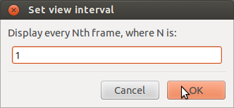
Before you start strokelitude, make sure that the display update interval is set to 1. During the recording, you may want to set this higher in order to be able to use lower values of “shutter (msec)” in the camera controls (i.e. a higher sampling rate). If you use a 10msec shutter with a display update interval of 1 it may happen that the program crashes. However, when you change settings in strokelitude, you should have a display update interval of 1, since the program might crash otherwise for unknown reasons.

To set the display update interval, go to “View” -> “Set display update interval…”.

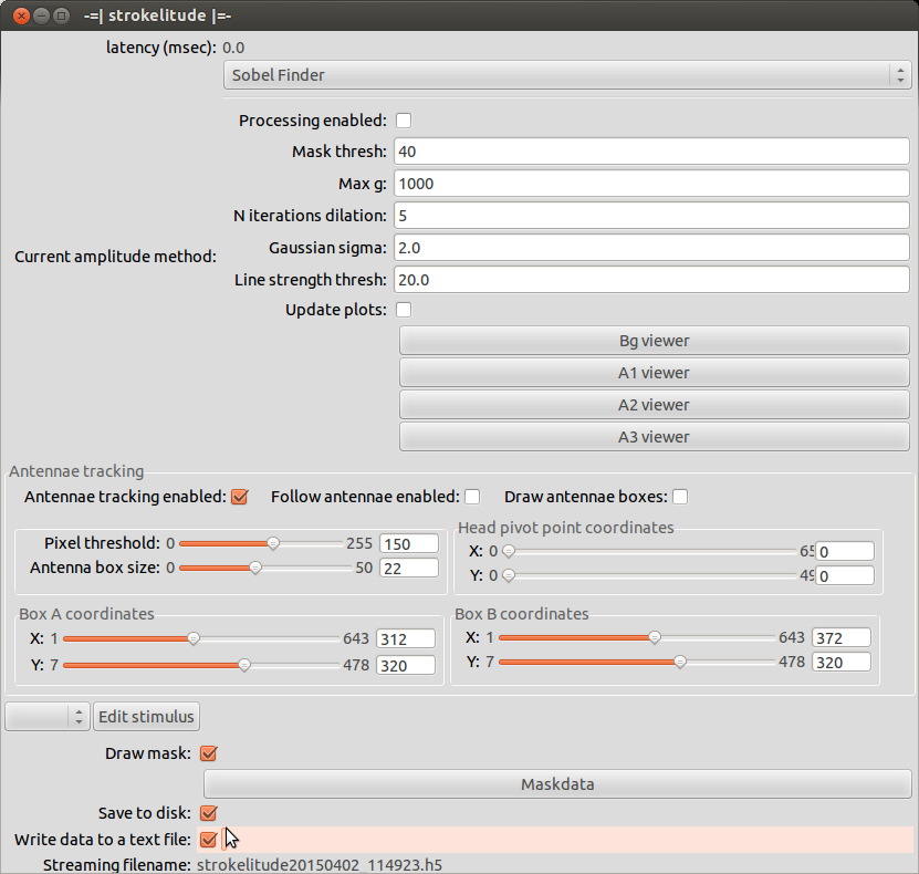
Open strokelitude. Go to “Windows” -> “-=|strokelitude|=-“. The click “Draw Mask”.

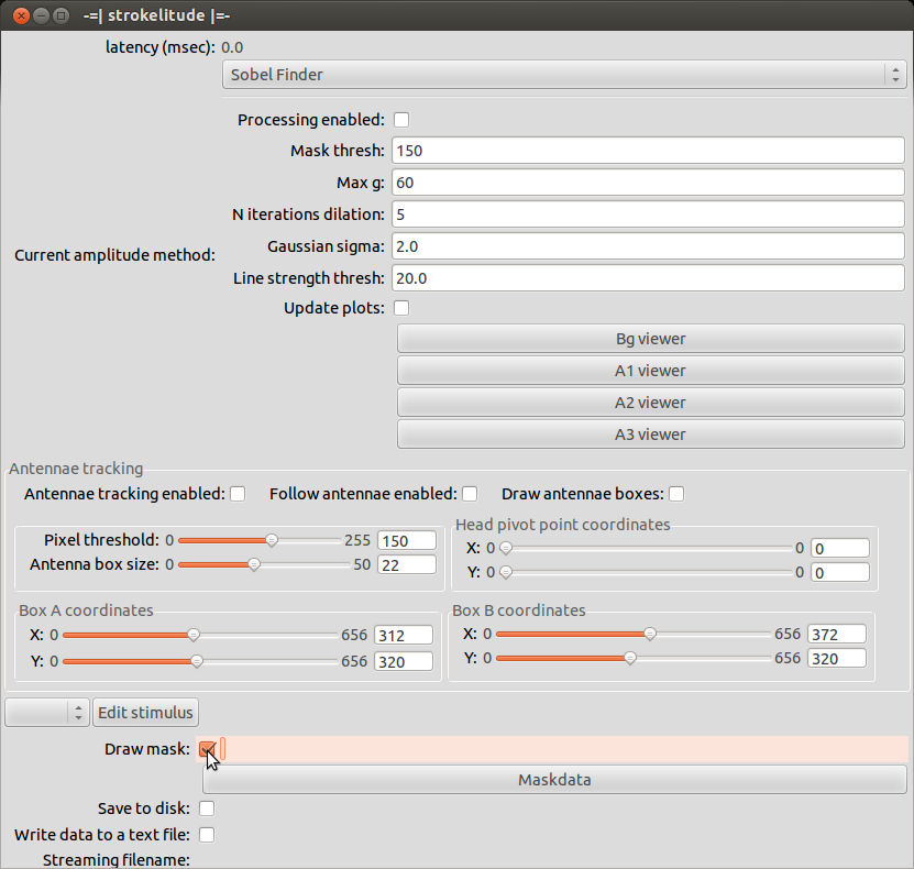
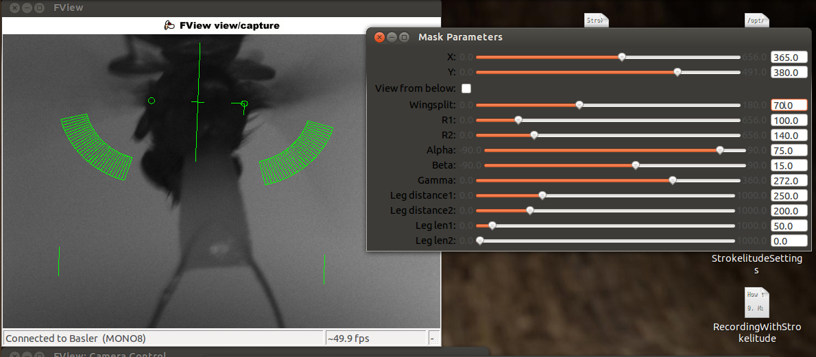
This will make some green lines appear on the screen. This is the mask for recording the fly. The two small circles should be on the roots of the wings and the line linking them should be orthogonal to the fly’s body axis (i.e. the orthogonal green line should be on the fly’s body axis). Unless you are very lucky (or very precise at fly handling), you will have to adjust the mask. To do this, click “Maskdata”. Another window will open.

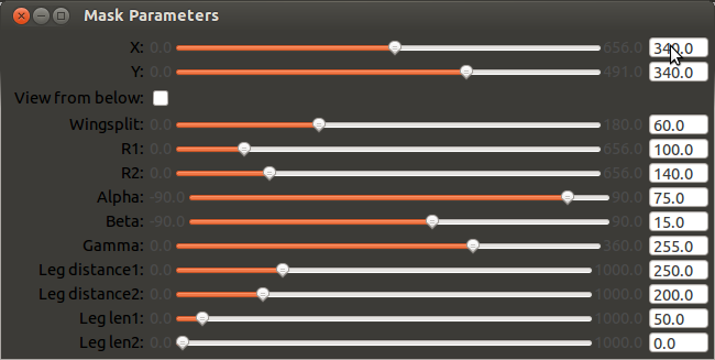
Use these parameters to fit the mask to the fly. With “gamma” you can rotate the mask and with “X” and “Y” you can shift it. Use these three parameters to position the two small circles to the wig hinges. You can manipulate the distance between the circles with “wingsplit”. Then you can use “R1” and “R2” to manipulate the inner and outer radii of the measurement sectors. With “alpha” and “beta” you can adjust the anterior and posterior borders of the measurement sectors. In general, these sectors should be positioned such that the anterior end of the wingstroke always falls inside. Optimally, nothing except for the wings should be within the sectors.

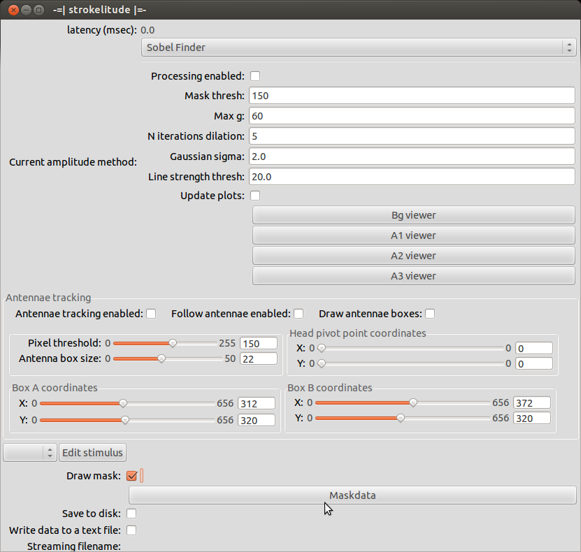
When you have set up the mask, close the window “Mask Parameters” and click “Antennae tracking enabled” in strokelitude.

This will make some more lines appear on the screen. Unless you are interested in tracking antenna movements, you can safely ignore those. Enabling antennae tracking is necessary, since strokelitude does not save the data otherwise.

As soon as you have enabled antennae tracking, you can set the display update interval back up, e.g. to 5. Now you can also set the “shutter (msec)” in the camera controls to the value you want to use during the recording (e.g. 10). This will change the brightness level of the video.

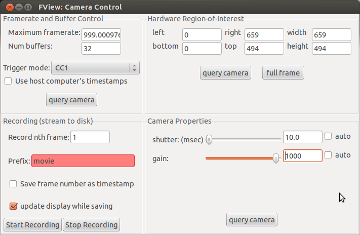
Turn on the infrared LED and put the filter in front of the camera (or adjust the lighting in whatever way is necessary for your experiment). Adjust the “gain” in the camera controls until you see a clear picture, where the wings of the fly are very bright and the background is very dark.

Go back to strokelitude and click “Processing enabled”.

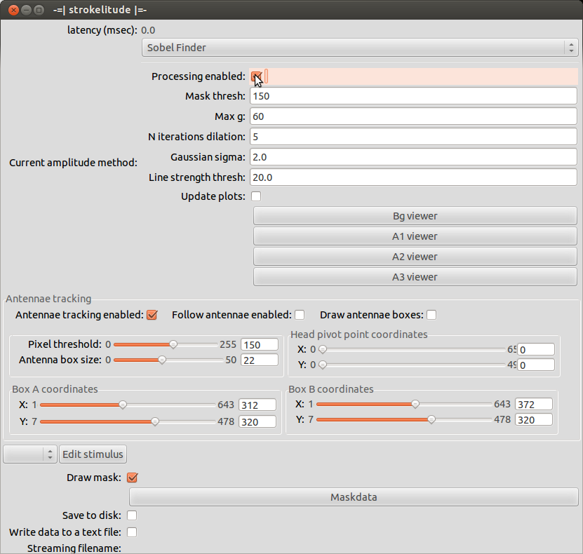
This will make two new green lines appear. They originate from the two small circles and go through the measurement sectors. These lines indicate the position that strokelitude calculates for the wing. This is the data you will record (even though you are not recording yet). Make sure that these lines track the wings well. Optimally, they should always be exactly on the border of the wing.

You can use “gain” to make the image brighter or darker. Also, the parameters “Mask thresh” and “Max g” (below the “Processing enabled” bottom in strokelitude) may be helpful. Raising max g may reduce the amount of error (frames in which strokelitude looses track of the wings). The mask threshold determines at which brightness level strokelitude estimates the border of he wing. As a rule of thumb, if the tracking lines jump down into the dark background area, you should raise the threshold. If the tracking lines jump up into the bright areas of the wing, you should lower the threshold.

However, pay attention to how homogeneous the wings are. Ideally, the wings should be a uniform white smear and the background should be black. If there is a bright stripe at the front of the wing and then a somewhat darker area behind it, this may lead to trouble, since strokelitude may switch between the two borders of the bright area. Sometimes it can help to put the measurement vectors further outside or further inside. Also, make sure that both wings are illuminated equally well, otherwise optimizing the settings for one wing will make you loose the other.

Once you made sure that strokelitude tracks the wings well, you can start the actual recording. Untick “Processing enabled” and select “Save to disk” (to save data in .h5 format) and “Write data to a text file” (to save data in .txt format). Then click “Processing enabled” to start the recording. If you want to record a video while you save the data, click “Start recording” in the camera controls.

Once you have finished the recording, disable processing. Find the data files, rename them and sort them (it is best to do this after every recording, since the file names strokelitude generates are generic). You can set the output directory under “File”. If you make several recordings, make sure to close fview between the sessions. Otherwise, strokelitude will continue to write the data into the same file.

Sathish data

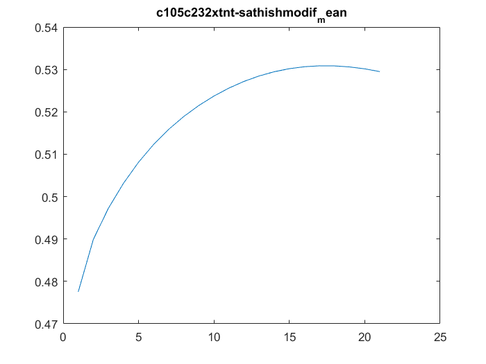
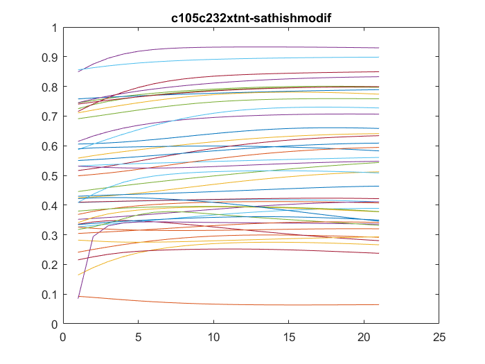
I have analyzed the c105+c232 > tnt data from Sathish. There are a total of 43 flies, although many of them only flew for a few minutes, and therefore should be discarded. Below all of the individual fly scores. I need to analyse now the other groups. This is btw the modified data set, whatever that means for Sathish.

This is a video of the projection from the torque data from Maye et al. 2007. The spikes are not that well sorted in this case as in the Strokelitude. I guess this is because the spikes do not look so smooth.

Recurrence quantitative analysis

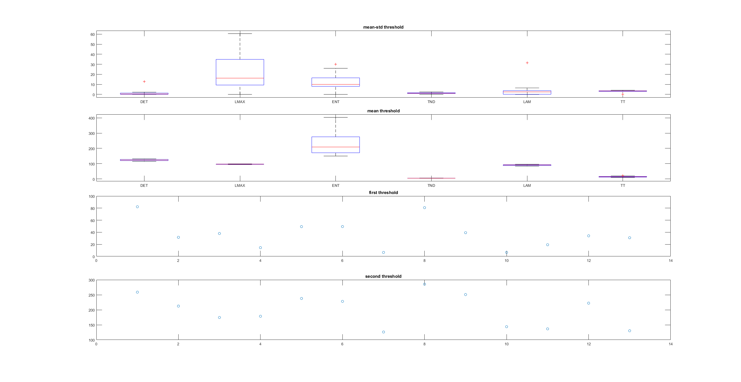
This is an example of a recurrence plot analysis. In the first graph is shown in single point in time in the optimal embedding dimension and the distance to the other points. For the recurrence plot analysis it is needed to put a threshold to make it binary. This is the second graph. From this second graph one can count many parameters like determinism, laminarity and so on. From what I see, the plots from the Strokelitude as well as Bjoern´s flight simulator in Maye et al 2007 show similar pattern (kind of crosses with vertical and horizontal lines).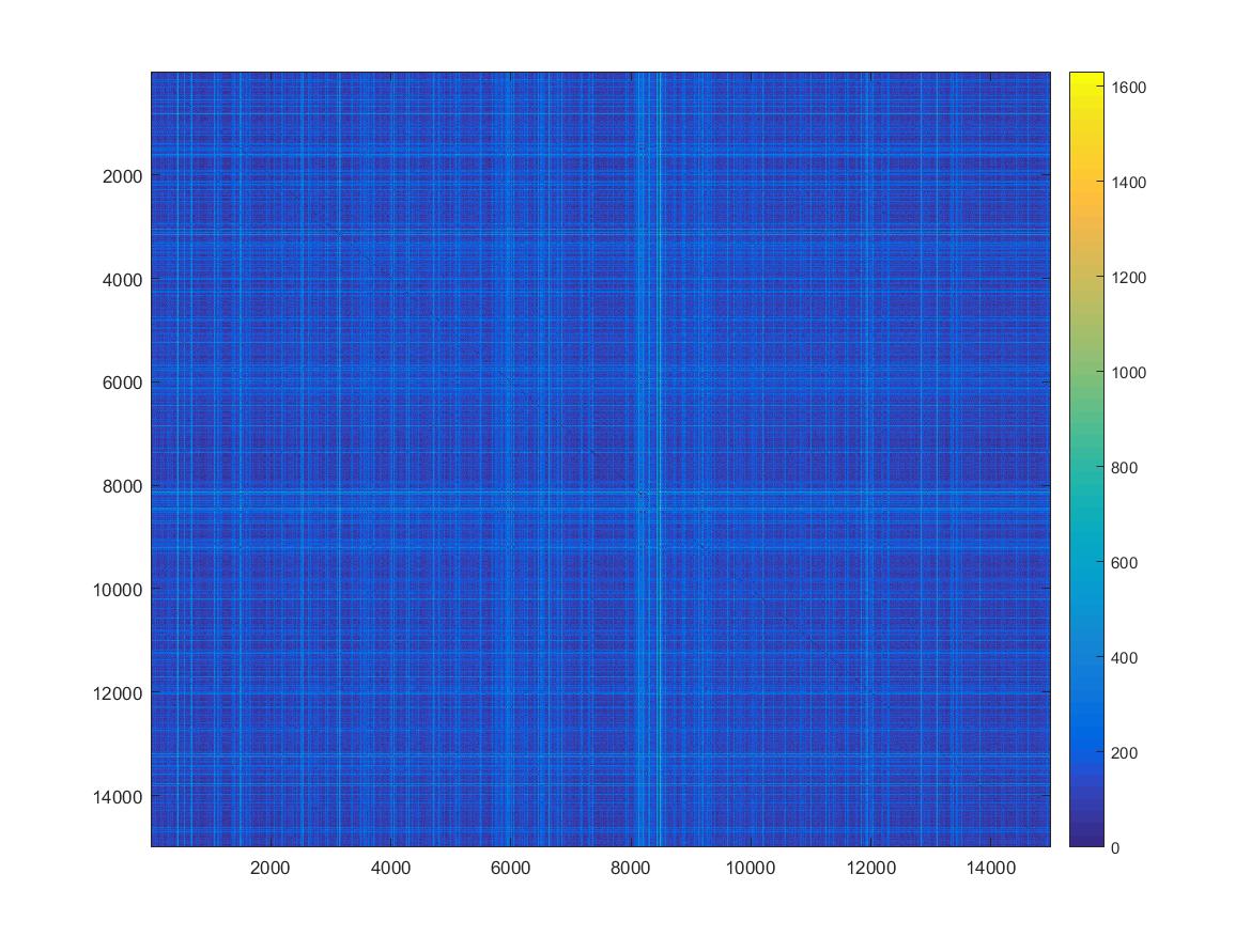

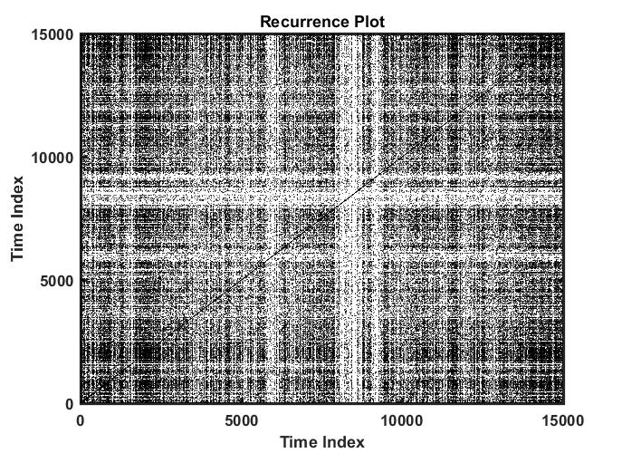
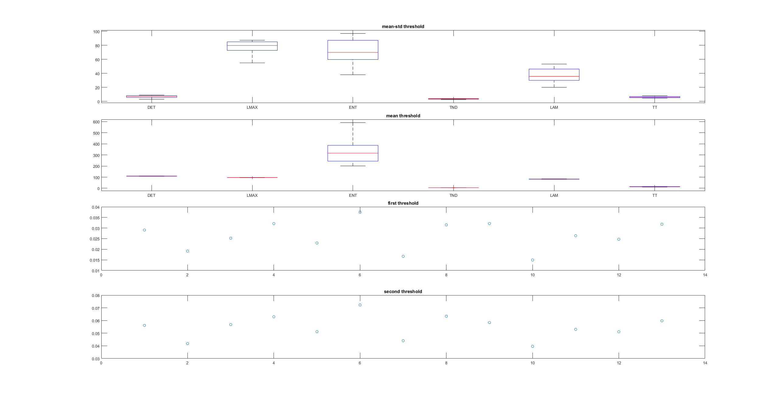
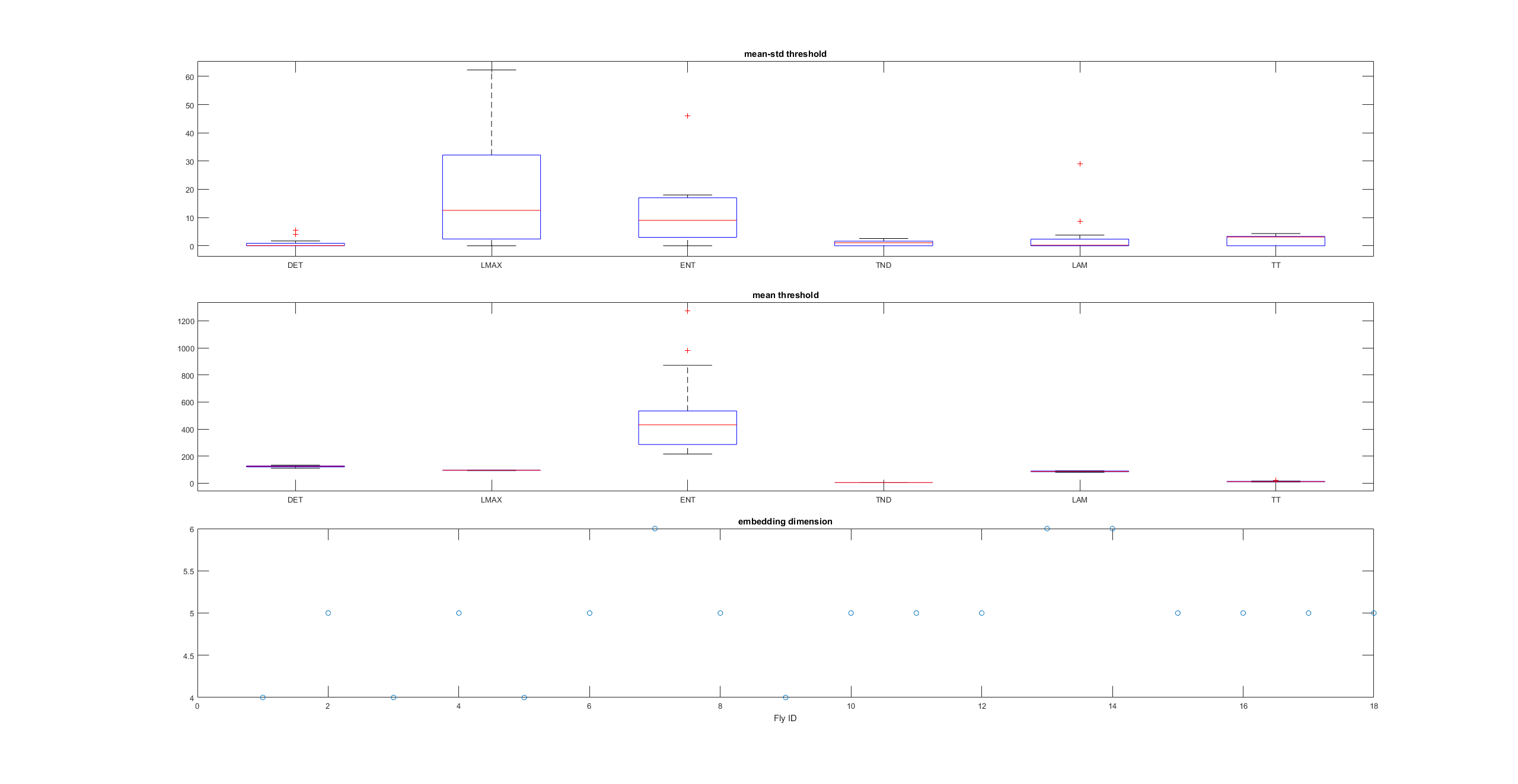
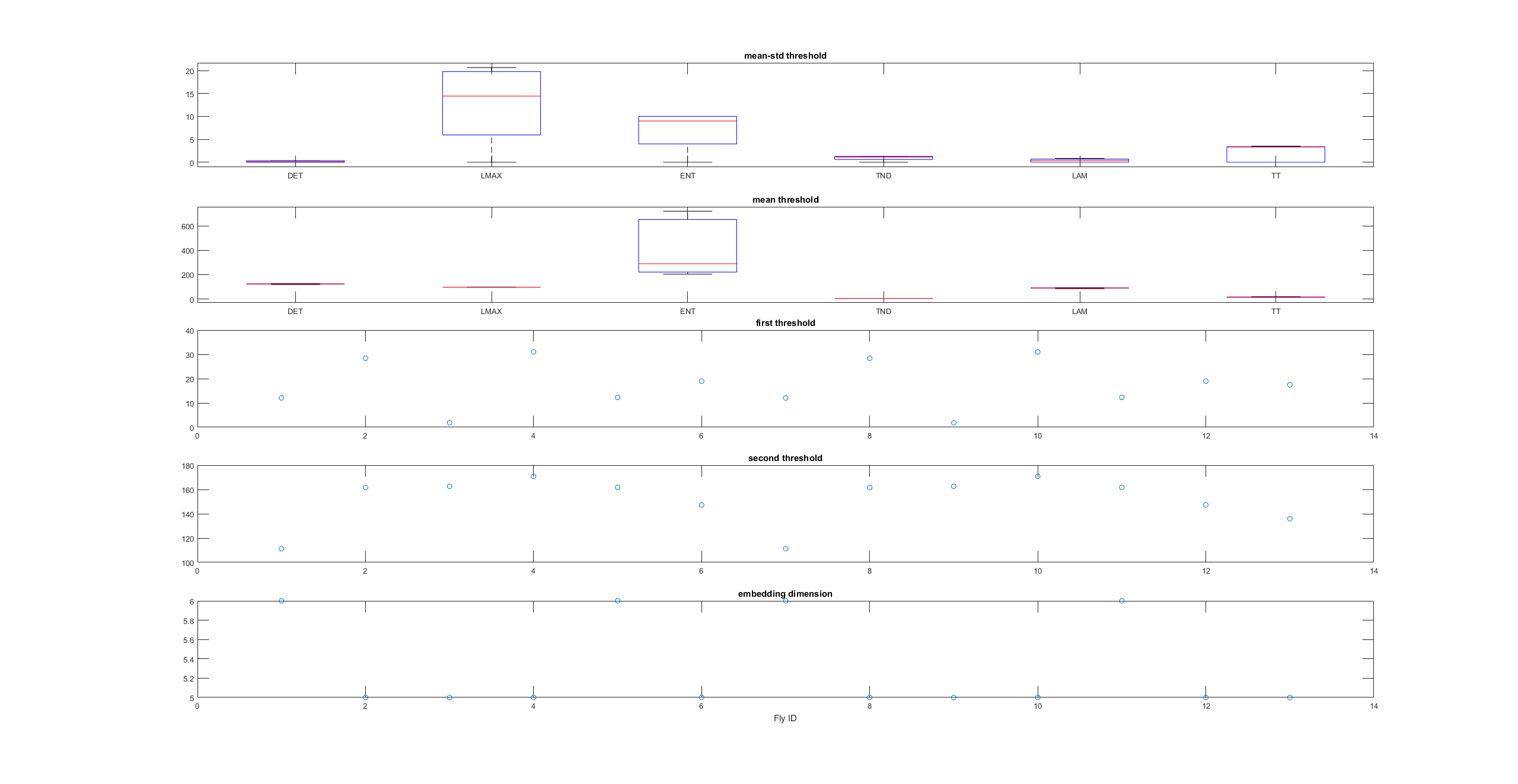
This is a measure of the Recurrence Quantitative Analysis of different groups. Recurrence threshold is a tricky and to some extent subjective measure, so this is why I tried two different ones.

DET: recurrence points that form a diagonal line of minimal length, the more diagonal, the more deterministic.

LMAX: Max diagonal line length or divergence. Sometimes considered as an estimator of max. Lyapunov exponent

ENT: Shannon entropy reflects the complexity of the system

TND: info about stationarity (trend)

LAM: Laminarity is related to laminar phases in the system (intermittency). It is tallied as vertical lines over a threshold.

TT: Trapping time, measuring the average length of vertical lines. Related to laminarity.

Automat

One stripe

Openloop

Uniform

Good bye Pablo!

After more than four months in our lab, we said good bye to Pablo Martinez (between Axel and Christian in the picture below).

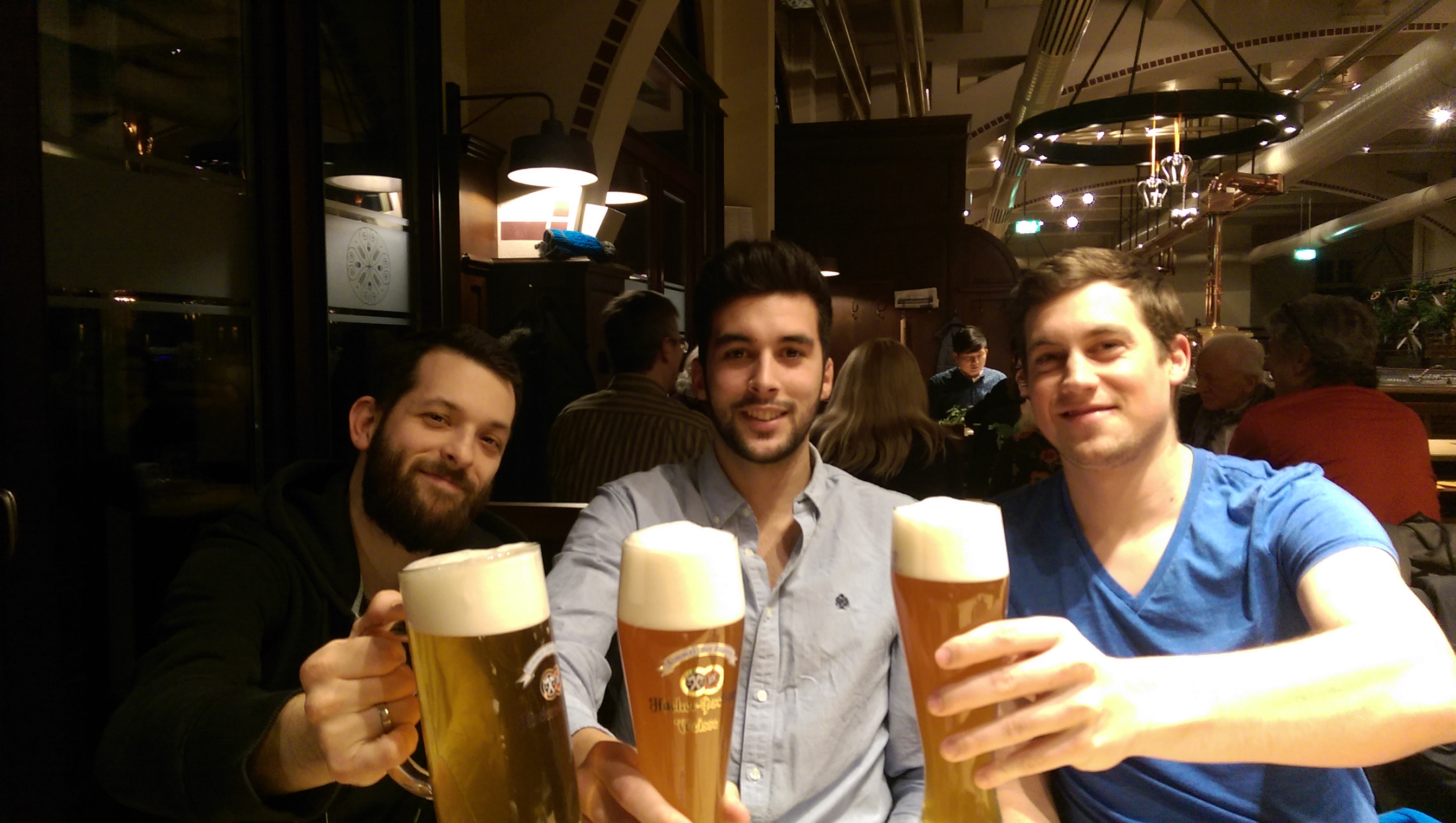He worked tirelessly to collect data on spontaneous flight behavior using strokelitude. We have enjoyed his visit tremendously and wish him all the best in his future research endeavors. Many thanks, Pablo!

The next students to leave the lab will be Amelie Roedel, Isabelle Steymans and Bianca Birk, who are writing up their theses right now.

First tests of fly prediction under a mean of the flies on single data points

These were done the week before last one but I could not upload it last time, so here are they. These are the results for predicting 4-5 flies of each group. Just one prediction from the middle of the time series for the 40 data points ahead in the future. First group is c105;;c232>TNT.

This is c105;;c232 x WTB

This is UAS-TNT x WTB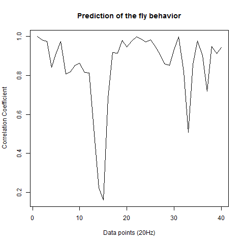

As I saw that the graph had so much zig-zag I told Pablo to make a bigger number of tested flies and this is what he is presenting today.

In addition I did analyze other parameters which are all saved under a PDF file below (Strokelitude). This contains some parameters with doubtfull processing which I still don´t trust so I have to find a better way for the calculation of it.

Strokelitude

Data analysis of the prediction of wingstroke amplitude with 40 datapoints.

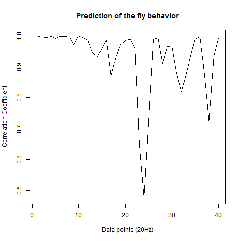
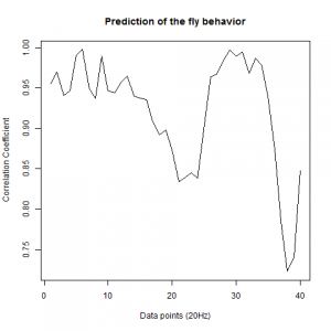
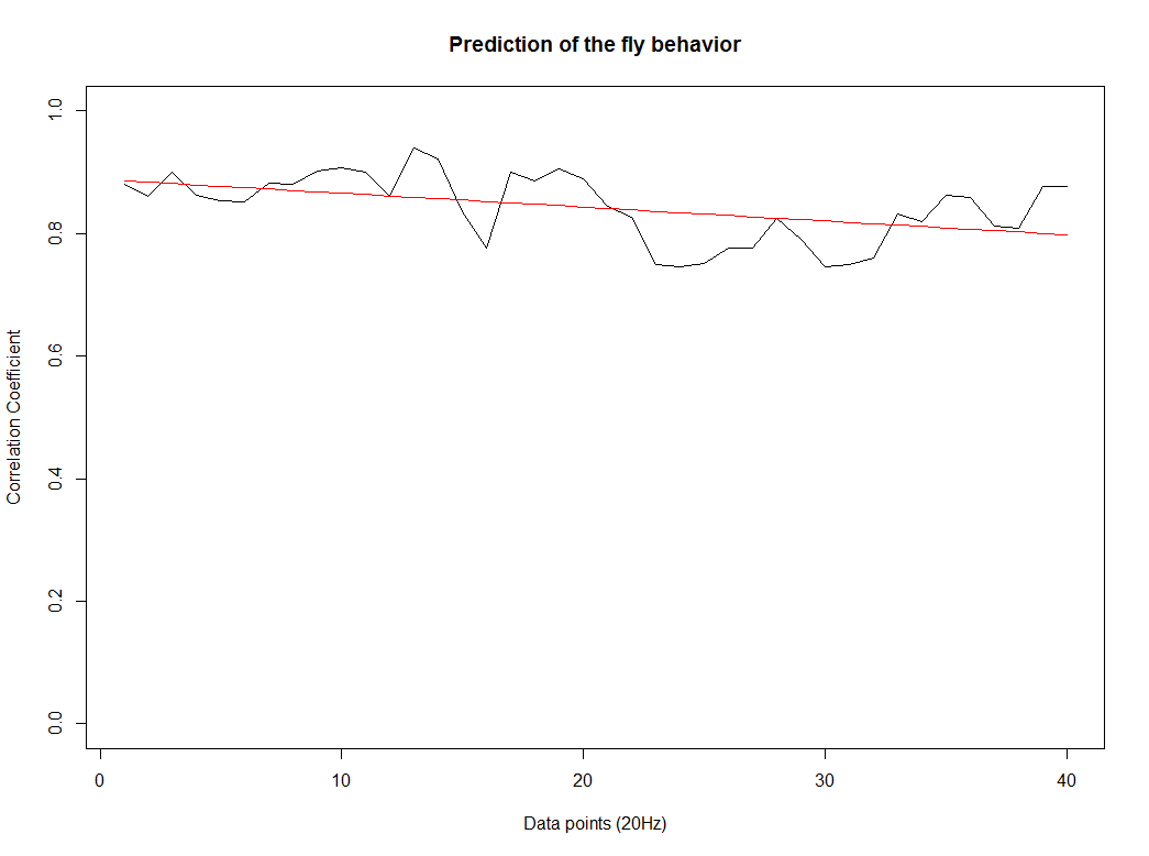
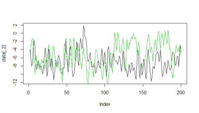
After we got the data of the behavior of the fly with strokelitude, we have made the analysis of 40 datapoints. Those datapoints were randomly picked in the middle of our dataset (10 minutes) and we made a second prediction, taking the points just before the end of the flight. For that we made a double correlation with those two predictions for each line and those are the results:

For the two control lines,

WTB x C105;;C232

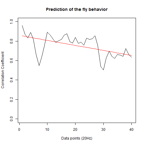
UAS-TNT-E x WTB

And for the experimental line (UAS-TNT-E x C105;;C232)

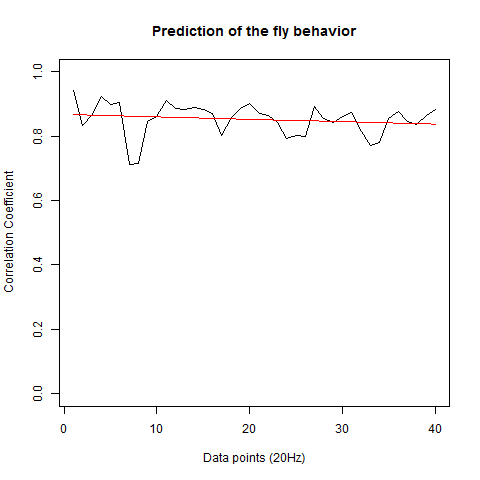
As long as the linear regresion decreases, more impredictable is the fly so its behave like non-linear function. The two controls are suposed to be more impredictable than the control line. There is more decrease in those two lines comparing to the experimental line, although is not too remarkable.

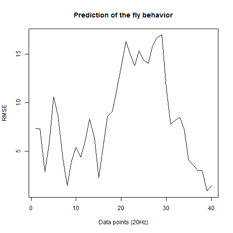
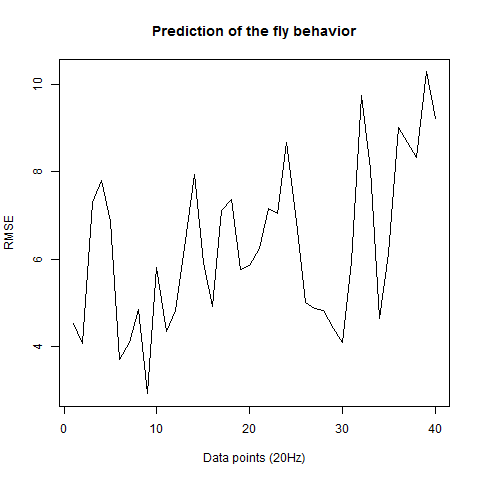
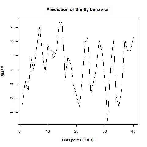
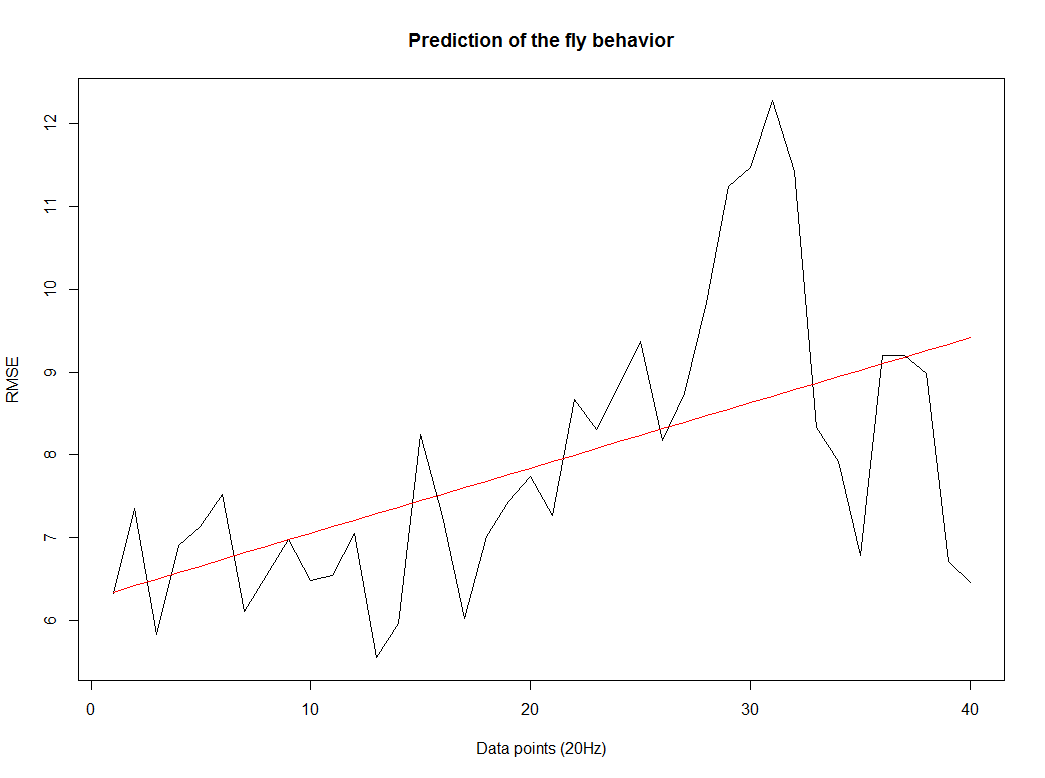
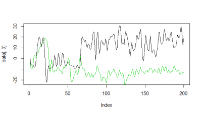
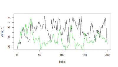
We also made an RMSE analysis, Christian explained it in his post. “RMSE measures just the differences of the absolute points whereas correlation coefficient is rather if the direction and degree of variation correlates (covariates)”

Here we have the plots:

WTB x C105;;C232(control)

UAS-TNT-E x WTB(control)

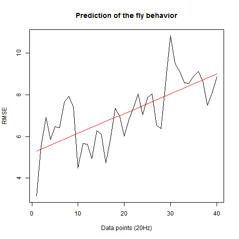
experimental line (UAS-TNT-E x C105;;C232)

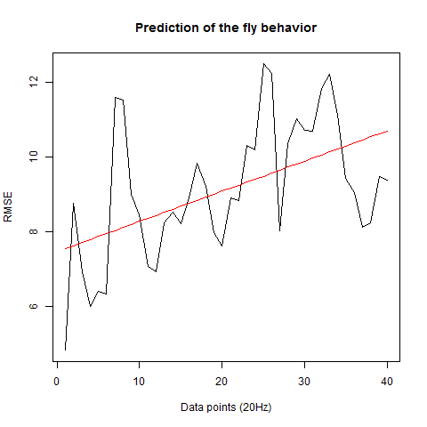
As long as the linear regresion increases, the absolute points differ from the prediction and the normal trace.

Prediction analysis

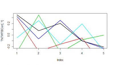
These are just 5 flies (WTBxTNT) from the strokelitude where I measured the correlation coefficient on the Y-axis. In the X-axis, first bin is from 0-2 s of prediction, second is 2-4s and so on.

It seems as if some flies do nicer than others. Although it seems to me that a correlation coefficient from 0.3 isnt a big thing with all this variability. I have to find out the best binning though, I think it needs to be much more in the short term.

When I do the mean of the 5 flies measured, I do see a very slight decay. But once more I would say the decay is from the bin 1 to the second.

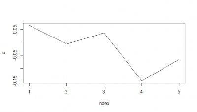
Here I tried another way, the RMSE, which according to literature and to my own reasoning should be a better analysis. I think RMSE measures just the differences of the absolute points whereas correlation coefficient is rather if the direction and degree of variation correlates (covariates). I find a very weird result. The fit is bad, the it gets better (but it should be just a chance event because correl coef decreases) and then it get very bad and so on.

I think for the future I have to make ensembles of two k neighbours maybe, which seem to increase the prediction power 10-15%. And maybe not look that much into the future as it was done here (10s).

Here some examples of predictions vs observations:

Protocols

Protocols

Preparing flies for Buridan’s Paradigm

T-maze (light vs dark)

T-maze phototaxis with LEDs

Phototaxis suppression

Sugar content in haemolymph

Benzer’s Countercurrent Apparatus

Installing fview and strokelitude

Measuring Wingstroke Amplitude with Strokelitude

Drosophila food preference assay