Searching interesting lines
on Friday, August 31st, 2018 4:23 | by Christian Rohrsen
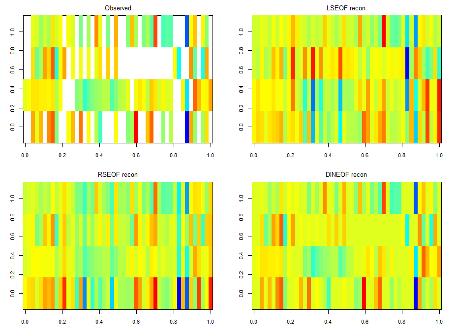
For finding if there are phenotype correlations in the different setups one needs a full matrix, which is not my case since I tested to some extent different lines in different setups. To make it more graphically, the observed results are shown in the above-left table. Colours just means values obtained (colorbars are unfortunately missing but it´s not so important) and each of the rows is a setup and each of the columns a fly line tested.
For testing correlations among setups, and similarly for doing a PCA one needs a full matrix, and not a sparse matrix as I have. What are the options? a few…
There is LSEOF (Empirical Orthogonal Function Analysis), RSEOF which is like LSEOF but recursive and normally achieves better results. There is another algorithm that is called DINEOF which consists of an additional step, interpolation, before doing LSEOF. The latter has shown to yield the best results. That is why I opted for this for filling my matrix for further analysis.
The results are shown in the figure below
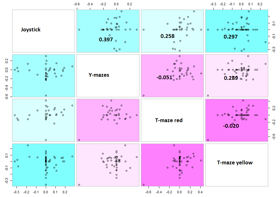
 Here the correlation of the mean results for the lines tested in the experiments. From the correlation numbers I would not say that there is any clear correlation of any experiment to the other ( Adj R² = 0.1392 for Joystick and Y-mazes; Adj R² = 0.06809 for Joystick and yellow T-maze)
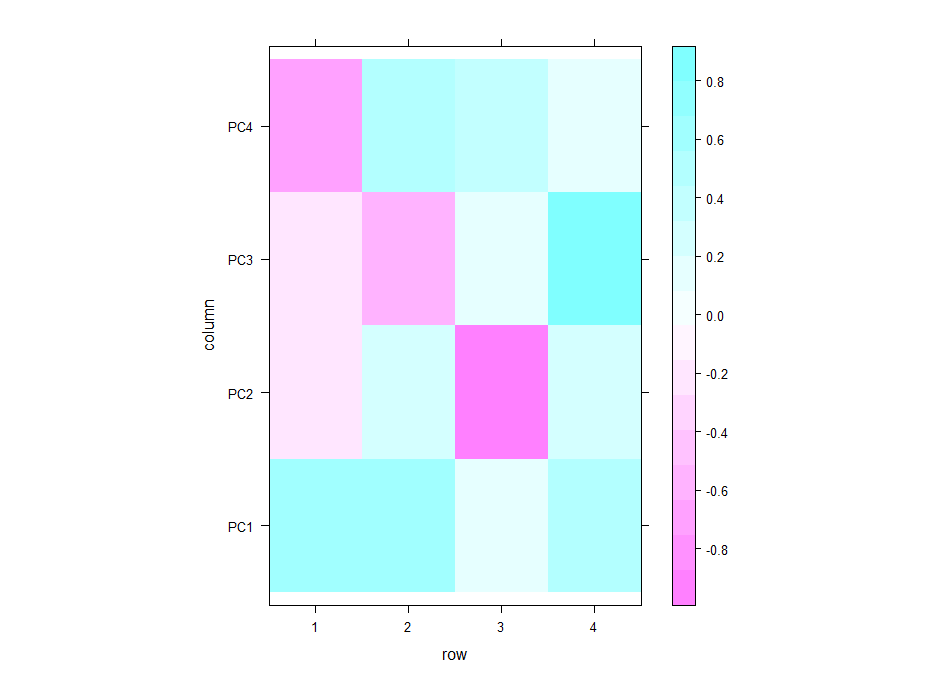
Even if there is no clear correlation among setups that the PCA could use, I decided to do a PCA to see what comes out of it. In the table below one can see the PCA loadings from the 4 different setup. We see that the PC1 uses a positive correlation of Joystick,Ymazes and yellow T-maze. PC2 a negative correlation of red T-maze and Joystick and positive Y-mazes and yellow T-mazes. After all there is not much to say about this, I think.
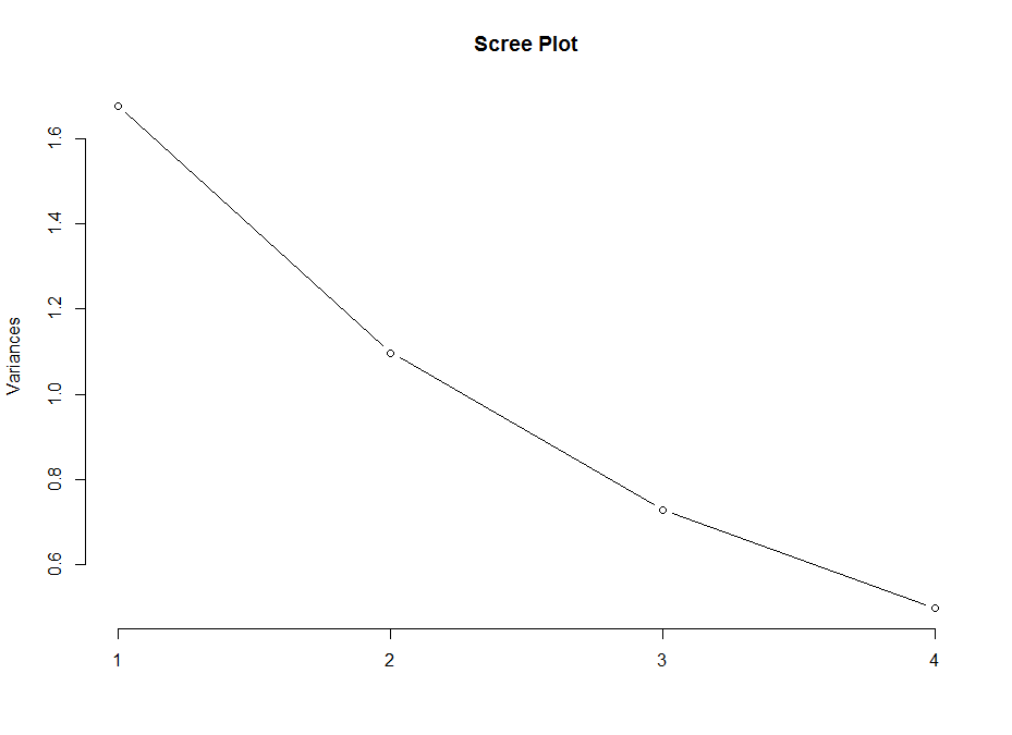
 This scree plot without any clear elbow gives me the impression that there is not much information here.
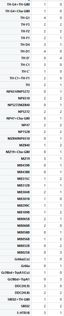
 This is how the table of “discrete phenotypes” looks like. The first column is positive scores and the second is negative scores. That means that we are looking for lines that have 4´s. This means that it has 4 negative/positive scores (Joystick, Ymazes, Tmaze red and yellow). In this case TH-G1 and TH-D1 have 4 positive scores (HL9 and TH-C1 have 3). TH-D’ have 4 negative scores (MB025B has 3). Unfortunately not all lines were tested in all setups so we might miss some interesting lines.
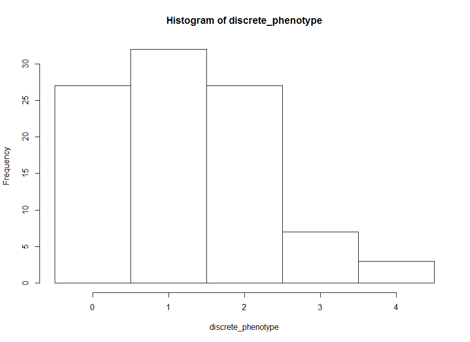
This is an histogram of the amount of zeros, ones,… that are in the above table.
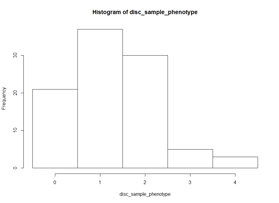
 The histogram below is the same as above but by generating surrogate data. I just sampled data from each experiment and checked what this imaginary lines might do. The histogram is quite similar to the one above. I think that having the same histogram shape only shows that there is not correlation of effects among setups, which was already shown above.
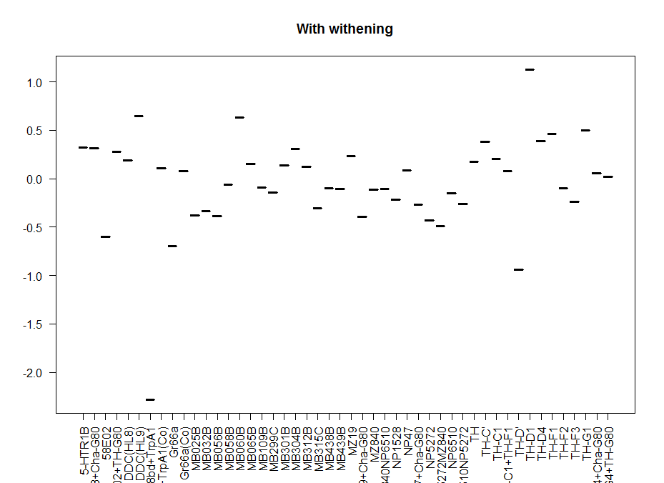
This is another way of looking for the interesting lines. I decided to withen the data so that all have mean zero and equal deviation so that all experiments have same weight. Then I did a mean for all experiments for each line. The extreme values show that they had a very strong overall phenotype. Here one can confirm what was seen with the “discrete phenotypes”. TH-D’ shows a negative score. TH-D1 a positive one, as well as MB060B and HL9.
Here we plot in different colours the effect from each of the setups tested. Here are also lines like TH-D’ and TH-D1 outstanding. I think it is important to see that the longer the bars the most interesting, but also the more mixed contribution of each experiment the more stronger the statistics might be.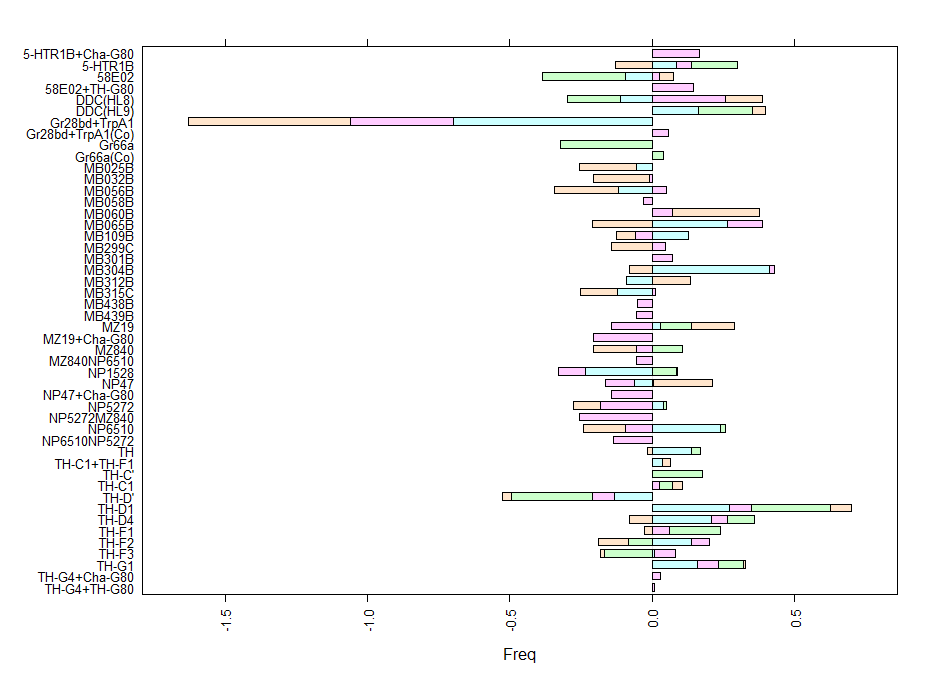

Category: neuronal activation, Operant reinforcment, Optogenetics
Leave a Reply